Label-aware subselection of echo data based on ship tracks

This notebook accompanies the following paper:

Echopype: Interoperable and scalable echosounder data processing with Echopype
Authors: Wu-Jung Lee, Landung Setiawan, Caesar Tuguinay, Emilio Mayorga, and Valentina Staneva
ICES Journal of Marine Science 2024: https://doi.org/10.1093/icesjms/fsae133

Introduction

Description

This notebook uses a small subset of the EK60 echosounder data collected during the 2017 Joint U.S.-Canada Integrated Ecosystem and Pacific Hake Acoustic Trawl Survey (aka the “Hake survey”) to illustrate how data processed from echosounder can be easily used with functions from core scientific Python software packages. Here, we use Xarray and GeoPandas to access and organize the ship position (GPS) data embedded in the echosounder dataset, and in turn use the ship track to slice (select) the echo data for plotting.

Outline

1. Connect with AWS S3 bucket and generate a list of target echosounder RAW files

2. Convert, calibrate, regrid, and save echosounder data as Zarr stores on disk

3. Regrid calibrated Sv data to MVBS

4. Extract and organize ship GPS data from the Platform group of the Zarr stores

5. Slice and plot echo data based on selected ship track segments

Running the notebook

This notebook can be run with a conda environment created using the conda environment file. The notebook creates a directory, if not already present: ./exports/ship_tracks. All Zarr files will be exported there.

Note

• We encourage importing Echopype as ep for consistency.

• Dask is not used in this notebook to parallelize the computation. Therefore, the cells may run a lot slower than those in krill_freq_diff.ipynb and OOI_eclipse.ipynb that also process similar volumes of data.

• combine_echodata, which allows users to combine and operate on echosounder data from multiple raw files as a single entity, is not used in this notebook. See OOI_eclipse.ipynb, krill_freq_diff.ipynb, and hake_mask.ipynb for its usage.

from pathlib import Path

import fsspec
import geopandas as gpd
import xarray as xr
import numpy as np

import matplotlib.pyplot as plt
from shapely.geometry import box
import cartopy.crs as ccrs
import cartopy.io.img_tiles as cimgt
from cartopy.mpl.gridliner import LONGITUDE_FORMATTER, LATITUDE_FORMATTER

import echopype as ep
from echopype.qc import exist_reversed_time

import warnings
warnings.simplefilter("ignore", category=DeprecationWarning)

Setup

Path setup

Set paths and create directories to store Zarr files:

output_path = Path("./exports/ship_tracks")
output_path.mkdir(exist_ok=True, parents=True)

echodata_zarr_path = output_path / "echodata_zarr"
echodata_zarr_path.mkdir(exist_ok=True)
Sv_zarr_path = output_path / "Sv_zarr"
Sv_zarr_path.mkdir(exist_ok=True)
MVBS_zarr_path = output_path / "MVBS_zarr"
MVBS_zarr_path.mkdir(exist_ok=True)

Processing echosounder data

Below we loop through all target .raw files to convert, calibrate, and regrid the data to generate mean volume backscattering strength (MVBS). We save intermediate data products to disk to enable out-of-core computation (when the computation may require resources larger than the system memory).

Connect with AWS S3 bucket and generate a list of target echosounder RAW files

Here, we access the public NOAA Water-Column Sonar Data Archive S3 bucket via the fsspec file system interface, to identify a list of EK60 .raw files to be processed in this notebook.

fs = fsspec.filesystem('s3', anon=True)

bucket = "ncei-wcsd-archive"
raw_path = "data/raw/Bell_M._Shimada/SH1707/EK60"

raw_files = fs.glob(f"{bucket}/{raw_path}/*.raw")

# print out the last two S3 raw file paths in the list for verification
raw_files[-2:]

['ncei-wcsd-archive/data/raw/Bell_M._Shimada/SH1707/EK60/Summer2017-D20170913-T180733.raw',
 'ncei-wcsd-archive/data/raw/Bell_M._Shimada/SH1707/EK60/Winter2017-D20170615-T002629.raw']

Generate list of target EK60 .raw files from AWS S3 bucket based on dates from July 28-29, 2017.

raw_files = [
    s3path for s3path in raw_files 
    if any([f"D2017{datestr}" in s3path for datestr in ['0728', '0729']])
]

print(f"There are {len(raw_files)} target raw files available")

There are 170 target raw files available

raw_files[0]

'ncei-wcsd-archive/data/raw/Bell_M._Shimada/SH1707/EK60/Summer2017-D20170728-T000534.raw'

Below is a function to (optionally) populate EchoData objects with NOAA Fisheries metadata about the Pacific Hake Survey. More information about the survey program is available at Joint U.S.-Canada Integrated Ecosystem and Pacific Hake Acoustic Trawl Survey.

def populate_metadata(ed, raw_fname):
    """
    Populate metadata about the dataset and survey platform
    into the EchoData object.
    """
    
    # -- SONAR-netCDF4 Top-level Group attributes
    survey_name = (
        "2017 Joint U.S.-Canada Integrated Ecosystem and "
        "Pacific Hake Acoustic Trawl Survey (the 'Hake survey')"
    )
    ed['Top-level'].attrs['title'] = f"{survey_name}, file {raw_fname}"
    ed['Top-level'].attrs['summary'] = (
        f"EK60 raw file {raw_fname} from the {survey_name}, "
        "converted to SONAR-netCDF4 using Echopype."
        "Information about the survey program is available at "
        "https://www.fisheries.noaa.gov/west-coast/science-data/"
        "joint-us-canada-integrated-ecosystem-and-pacific-hake-acoustic-trawl-survey"
    )

    # -- SONAR-netCDF4 Platform Group attributes
    # Per SONAR-netCDF4, for platform_type see https://vocab.ices.dk/?ref=311
    ed['Platform'].attrs['platform_type'] = "Research vessel"
    ed['Platform'].attrs['platform_name'] = "Bell M. Shimada"  # A NOAA ship
    ed['Platform'].attrs['platform_code_ICES'] = "315"

Convert, calibrate, regrid, and save echosounder data as Zarr stores on disk

Depending on your internet speed, this cell below may take some time to run (potentially 20-30 mins).

%%time

for rf in raw_files:
    raw_fpath = Path(rf)
    try:
        # Access file directly from S3 to create a converted EchoData object in memory
        ed = ep.open_raw(
            f"s3://{rf}",
            sonar_model="EK60",
            use_swap=True,
            storage_options={"anon": True}
        )
        # Populate additional metadata
        populate_metadata(ed, raw_fpath.name)

        # Save to the converted EchoData object to Zarr on disk
        ed.to_zarr(save_path=echodata_zarr_path, overwrite=True)

        # Calibrate raw backscatter measurement to Sv 
        ds_Sv = ep.calibrate.compute_Sv(ed)

        # Add depth to the Sv dataset
        ds_Sv = ep.consolidate.add_depth(ds_Sv, depth_offset=9.15)

        # Save Sv dataset to Zarr on disk
        ds_Sv.to_zarr(Sv_zarr_path / f"{raw_fpath.stem}_Sv.zarr", mode="w")

    except Exception as e:
        print(f"Failed to process raw file {raw_fpath.name}: {e}")

CPU times: user 5min 22s, sys: 1min 34s, total: 6min 57s
Wall time: 10min 32s

Below we regrid Sv data by computing mean volume backscattering strength (MVBS), which are binned averages of Sv (in the linear domain) across ping time and depth. Note that we take extra care in slicing the combined Sv store so that the ping_time intervals does not overlap for successive MVBS bins.

Note: The workflow in this notebook differs from the approaches used in the other two notebooks that also utilize the 2017 Hake survey data (hake_NASC_EK60.ipynb and krill_NASC_EK60.ipynb).

In the mentioned notebooks, the .raw files are converted into EchoData objects individually. These objects are then combined using combine_echodata, with subsequent calibration and regridding performed on the combined EchoData object.

In contrast, this notebook handles the conversion, calibration, and regridding of each .raw file separately. We show this workflow variant to demonstrate the flexibility of using Echopype functions.

Regrid calibrated Sv data to MVBS

%%time

# Grab and sort Sv zarr paths
Sv_zarr_path_list = list(Sv_zarr_path.glob('*.zarr'))
Sv_zarr_path_list.sort()

# Initialize leftover ds_Sv zarr as None
leftover_ds_Sv = None

# Iterate through all Sv Zarr Paths
for file_path in Sv_zarr_path_list:
    # Open ds_Sv from disk Zarr
    ds_Sv = xr.open_zarr(file_path)

    # Concat leftover Sv with current Sv
    if leftover_ds_Sv is not None:
        concat_ds_Sv = xr.concat([leftover_ds_Sv, ds_Sv], dim="ping_time")
    else:
        concat_ds_Sv = ds_Sv
    
    # Resample data into 20-second bins
    resampled_data = concat_ds_Sv.resample(ping_time="20s", skipna=True)

    # Determine the start index of the last incomplete 20-second bin
    cutoff_index = max(group.start for group in resampled_data.groups.values())

    # Split data into complete and incomplete bins:

    # Take data up to the last complete bin
    complete_bins_Sv = concat_ds_Sv.isel(ping_time=slice(0, cutoff_index))

    # Keep remaining data for next iteration
    leftover_ds_Sv = concat_ds_Sv.isel(ping_time=slice(cutoff_index, None))

    # Compute MVBS on current subset
    ds_MVBS = ep.commongrid.compute_MVBS(
        complete_bins_Sv,
        range_var="depth",
        range_bin='5m',  # in meters
        ping_time_bin='20s',  # in seconds
    )

    # Save MVBS dataset to Zarr on disk
    ds_MVBS.to_zarr(MVBS_zarr_path / f"{file_path.stem.replace('Sv', 'MVBS')}.zarr", mode="w")

CPU times: user 5min 37s, sys: 2min 33s, total: 8min 10s
Wall time: 7min 18s

We now check that each ping time bin is unique across all MVBS Zarr Stores:

%%time

# Iterate through MVBS Zarr Stores
for file_path in MVBS_zarr_path.glob('*.zarr'):
    # Grab ping times from MVBS Zarr Store
    ping_times = xr.open_zarr(file_path)["ping_time"].values

    # Check that all ping times are unique
    assert len(np.unique(ping_times)) == len(ping_times)

CPU times: user 663 ms, sys: 11.3 ms, total: 674 ms
Wall time: 674 ms

Test for time reversals

Small time reversals are sometimes found in EK60 datasets, where some ping_time (or GPS time1) value may be lower (older) than the preceding ping_time. Such discontinuities can interfere with concatenating data from individual files to produce an aggregated dataset. This issues can be identified and addressed by functions in the echopype.qc subpackage.

for filepath in echodata_zarr_path.glob('*.zarr'):
    ed = ep.open_converted(filepath)
    # Test for a negative ping_time increment in sequential timestamps, in the Sonar/Beam_group1 group
    if exist_reversed_time(ds=ed['Sonar/Beam_group1'], time_name='ping_time'):
        print(f'Reversed time in {filepath}')

There are no time reversals in this two-day dataset, fortunately.

Extract and organize ship GPS data from the Platform group of the Zarr stores

Below we will use the Xarray open_mfdataset function to open and concatenate data from the Platform group from all converted EchoData Zarr stores, then assemble the GPS data (timestamp, latitude, and longitude) into a GeoPandas GeoDataFrame containing point-geometry objects. Note that GeoDataFrame adds geospatial capabilities to regular Pandas DataFrame.

Due to the presence of multiple time coordinates in the Platform group, we are careful in the argument passed to open_mfdataset to ensure the catenation for different variables is along the right coordinates.

%%time
ds_platform = xr.open_mfdataset(
    str(echodata_zarr_path / '*.zarr'),
    group='Platform', 
    engine='zarr',
    data_vars='minimal', coords='minimal',
    combine='nested',
    chunks='auto',
)

CPU times: user 48.9 s, sys: 2.38 s, total: 51.3 s
Wall time: 51.1 s

ds_platform

<xarray.Dataset> Size: 11MB
Dimensions:              (channel: 3, time1: 244846, time2: 88959)
Coordinates:
  * channel              (channel) <U37 444B 'GPT  18 kHz 009072058c8d 1-1 ES...
  * time1                (time1) datetime64[ns] 2MB 2017-07-28T00:05:36.10331...
  * time2                (time2) datetime64[ns] 712kB 2017-07-28T00:05:34.897...
Data variables: (12/20)
    MRU_offset_x         float64 8B nan
    MRU_offset_y         float64 8B nan
    MRU_offset_z         float64 8B nan
    MRU_rotation_x       float64 8B nan
    MRU_rotation_y       float64 8B nan
    MRU_rotation_z       float64 8B nan
    ...                   ...
    sentence_type        (time1) object 2MB dask.array<chunksize=(244846,), meta=np.ndarray>
    transducer_offset_x  (channel) float64 24B dask.array<chunksize=(3,), meta=np.ndarray>
    transducer_offset_y  (channel) float64 24B dask.array<chunksize=(3,), meta=np.ndarray>
    transducer_offset_z  (channel) float64 24B dask.array<chunksize=(3,), meta=np.ndarray>
    vertical_offset      (time2) float64 712kB dask.array<chunksize=(88959,), meta=np.ndarray>
    water_level          float64 8B 9.15
Attributes:
    platform_code_ICES:  315
    platform_name:       Bell M. Shimada
    platform_type:       Research vessel

xarray.Dataset

• Dimensions:
  • channel: 3
  • time1: 244846
  • time2: 88959
• Coordinates: (3)
  • channel
    (channel)
    <U37
    'GPT 18 kHz 009072058c8d 1-1 ES...

    long_name :

    Vendor channel ID

    array(['GPT  18 kHz 009072058c8d 1-1 ES18-11',
           'GPT  38 kHz 009072058146 2-1 ES38B',
           'GPT 120 kHz 00907205a6d0 4-1 ES120-7C'], dtype='<U37')

  • time1
    (time1)
    datetime64[ns]
    2017-07-28T00:05:36.103315 ... 2...

    axis :

    T

    comment :

    Time coordinate corresponding to NMEA position data.

    long_name :

    Timestamps for NMEA datagrams

    standard_name :

    time

    array(['2017-07-28T00:05:36.103315000', '2017-07-28T00:05:37.511097000',
           '2017-07-28T00:05:37.669428000', ..., '2017-07-30T00:17:57.274191000',
           '2017-07-30T00:17:59.223482000', '2017-07-30T00:17:59.381813000'],
          dtype='datetime64[ns]')

  • time2
    (time2)
    datetime64[ns]
    2017-07-28T00:05:34.897272 ... 2...

    axis :

    T

    comment :

    Time coordinate corresponding to platform motion and orientation data.

    long_name :

    Timestamps for platform motion and orientation data

    standard_name :

    time

    array(['2017-07-28T00:05:34.897272000', '2017-07-28T00:05:37.162401000',
           '2017-07-28T00:05:38.404472000', ..., '2017-07-30T00:17:52.050917000',
           '2017-07-30T00:17:54.266043000', '2017-07-30T00:17:56.492170000'],
          dtype='datetime64[ns]')

• Data variables: (20)
  • MRU_offset_x
    ()
    float64
    nan

    long_name :

    Distance along the x-axis from the platform coordinate system origin to the motion reference unit sensor origin

    units :

    m

    array(nan)

  • MRU_offset_y
    ()
    float64
    nan

    long_name :

    Distance along the y-axis from the platform coordinate system origin to the motion reference unit sensor origin

    units :

    m

    array(nan)

  • MRU_offset_z
    ()
    float64
    nan

    long_name :

    Distance along the z-axis from the platform coordinate system origin to the motion reference unit sensor origin

    units :

    m

    array(nan)

  • MRU_rotation_x
    ()
    float64
    nan

    long_name :

    Extrinsic rotation about the x-axis from the platform to MRU coordinate systems

    units :

    arc_degree

    valid_range :

    (–180.0, 180.0)

    array(nan)

  • MRU_rotation_y
    ()
    float64
    nan

    long_name :

    Extrinsic rotation about the y-axis from the platform to MRU coordinate systems

    units :

    arc_degree

    valid_range :

    (–180.0, 180.0)

    array(nan)

  • MRU_rotation_z
    ()
    float64
    nan

    long_name :

    Extrinsic rotation about the z-axis from the platform to MRU coordinate systems

    units :

    arc_degree

    valid_range :

    (–180.0, 180.0)

    array(nan)

  • frequency_nominal
    (channel)
    float64
    dask.array<chunksize=(3,), meta=np.ndarray>

    long_name :

    Transducer frequency

    standard_name :

    sound_frequency

    units :

    Hz

    valid_min :

    0.0

    Array Chunk Bytes 24 B 24 B Shape (3,) (3,) Dask graph 1 chunks in 845 graph layers Data type float64 numpy.ndarray

  • latitude
    (time1)
    float64
    dask.array<chunksize=(244846,), meta=np.ndarray>

    long_name :

    Platform latitude

    standard_name :

    latitude

    units :

    degrees_north

    valid_range :

    (-90.0, 90.0)

    Array Chunk Bytes 1.87 MiB 1.87 MiB Shape (244846,) (244846,) Dask graph 1 chunks in 1690 graph layers Data type float64 numpy.ndarray

  • longitude
    (time1)
    float64
    dask.array<chunksize=(244846,), meta=np.ndarray>

    long_name :

    Platform longitude

    standard_name :

    longitude

    units :

    degrees_east

    valid_range :

    (-180.0, 180.0)

    Array Chunk Bytes 1.87 MiB 1.87 MiB Shape (244846,) (244846,) Dask graph 1 chunks in 1690 graph layers Data type float64 numpy.ndarray

  • pitch
    (time2)
    float64
    dask.array<chunksize=(88959,), meta=np.ndarray>

    long_name :

    Platform pitch

    standard_name :

    platform_pitch_angle

    units :

    arc_degree

    valid_range :

    (-90.0, 90.0)

    Array Chunk Bytes 694.99 kiB 694.99 kiB Shape (88959,) (88959,) Dask graph 1 chunks in 1690 graph layers Data type float64 numpy.ndarray

  • position_offset_x
    ()
    float64
    nan

    long_name :

    Distance along the x-axis from the platform coordinate system origin to the latitude/longitude sensor origin

    units :

    m

    array(nan)

  • position_offset_y
    ()
    float64
    nan

    long_name :

    Distance along the y-axis from the platform coordinate system origin to the latitude/longitude sensor origin

    units :

    m

    array(nan)

  • position_offset_z
    ()
    float64
    nan

    long_name :

    Distance along the z-axis from the platform coordinate system origin to the latitude/longitude sensor origin

    units :

    m

    array(nan)

  • roll
    (time2)
    float64
    dask.array<chunksize=(88959,), meta=np.ndarray>

    long_name :

    Platform roll

    standard_name :

    platform_roll_angle

    units :

    arc_degree

    valid_range :

    (-90.0, 90.0)

    Array Chunk Bytes 694.99 kiB 694.99 kiB Shape (88959,) (88959,) Dask graph 1 chunks in 1690 graph layers Data type float64 numpy.ndarray

  • sentence_type
    (time1)
    object
    dask.array<chunksize=(244846,), meta=np.ndarray>

    long_name :

    NMEA sentence type

    Array Chunk Bytes 1.87 MiB 1.87 MiB Shape (244846,) (244846,) Dask graph 1 chunks in 1859 graph layers Data type object numpy.ndarray

  • transducer_offset_x
    (channel)
    float64
    dask.array<chunksize=(3,), meta=np.ndarray>

    long_name :

    x-axis distance from the platform coordinate system origin to the sonar transducer

    units :

    m

    Array Chunk Bytes 24 B 24 B Shape (3,) (3,) Dask graph 1 chunks in 845 graph layers Data type float64 numpy.ndarray

  • transducer_offset_y
    (channel)
    float64
    dask.array<chunksize=(3,), meta=np.ndarray>

    long_name :

    y-axis distance from the platform coordinate system origin to the sonar transducer

    units :

    m

    Array Chunk Bytes 24 B 24 B Shape (3,) (3,) Dask graph 1 chunks in 845 graph layers Data type float64 numpy.ndarray

  • transducer_offset_z
    (channel)
    float64
    dask.array<chunksize=(3,), meta=np.ndarray>

    long_name :

    z-axis distance from the platform coordinate system origin to the sonar transducer

    units :

    m

    Array Chunk Bytes 24 B 24 B Shape (3,) (3,) Dask graph 1 chunks in 845 graph layers Data type float64 numpy.ndarray

  • vertical_offset
    (time2)
    float64
    dask.array<chunksize=(88959,), meta=np.ndarray>

    long_name :

    Platform vertical offset from nominal water level

    units :

    m

    Array Chunk Bytes 694.99 kiB 694.99 kiB Shape (88959,) (88959,) Dask graph 1 chunks in 1690 graph layers Data type float64 numpy.ndarray

  • water_level
    ()
    float64
    9.15

    long_name :

    Distance from the platform coordinate system origin to the nominal water level along the z-axis

    units :

    m

    array(9.14999962)

• Indexes: (3)
  • channel
    PandasIndex

    PandasIndex(Index(['GPT  18 kHz 009072058c8d 1-1 ES18-11',
           'GPT  38 kHz 009072058146 2-1 ES38B',
           'GPT 120 kHz 00907205a6d0 4-1 ES120-7C'],
          dtype='object', name='channel'))

  • time1
    PandasIndex

    PandasIndex(DatetimeIndex(['2017-07-28 00:05:36.103315', '2017-07-28 00:05:37.511097',
                   '2017-07-28 00:05:37.669428', '2017-07-28 00:05:37.948589',
                   '2017-07-28 00:05:39.000582', '2017-07-28 00:05:39.158913',
                   '2017-07-28 00:05:40.353559', '2017-07-28 00:05:41.152784',
                   '2017-07-28 00:05:41.311115', '2017-07-28 00:05:42.003654',
                   ...
                   '2017-07-30 00:17:52.538342', '2017-07-30 00:17:53.276962',
                   '2017-07-30 00:17:53.926178', '2017-07-30 00:17:54.084509',
                   '2017-07-30 00:17:55.277079', '2017-07-30 00:17:55.924213',
                   '2017-07-30 00:17:56.082544', '2017-07-30 00:17:57.274191',
                   '2017-07-30 00:17:59.223482', '2017-07-30 00:17:59.381813'],
                  dtype='datetime64[ns]', name='time1', length=244846, freq=None))

  • time2
    PandasIndex

    PandasIndex(DatetimeIndex(['2017-07-28 00:05:34.897272', '2017-07-28 00:05:37.162401',
                   '2017-07-28 00:05:38.404472', '2017-07-28 00:05:40.670601',
                   '2017-07-28 00:05:42.906729', '2017-07-28 00:05:45.152857',
                   '2017-07-28 00:05:47.387985', '2017-07-28 00:05:49.643114',
                   '2017-07-28 00:05:51.899244', '2017-07-28 00:05:54.145372',
                   ...
                   '2017-07-30 00:17:36.490026', '2017-07-30 00:17:38.716152',
                   '2017-07-30 00:17:40.951281', '2017-07-30 00:17:43.178410',
                   '2017-07-30 00:17:45.393536', '2017-07-30 00:17:47.619663',
                   '2017-07-30 00:17:49.835791', '2017-07-30 00:17:52.050917',
                   '2017-07-30 00:17:54.266043', '2017-07-30 00:17:56.492170'],
                  dtype='datetime64[ns]', name='time2', length=88959, freq=None))

• Attributes: (3)

  platform_code_ICES :

  315

  platform_name :

  Bell M. Shimada

  platform_type :

  Research vessel

We can use time1 (the timestamps for NMEA datagrams, or GPS timestamps) to examine the exact timestamp interval spanned by the combined dataset.

print(f"{ds_platform.time1.values.min()}, {ds_platform.time1.values.max()}")

2017-07-28T00:05:36.103315000, 2017-07-30T00:17:59.381813000

To organize the GPS data, we first create a Pandas DataFrame and then turn it into a GeoPandas GeoDataFrame.

df_gps = ds_platform.latitude.to_dataframe().join(ds_platform.longitude.to_dataframe())

df_gps.head(3)

	latitude	longitude
time1
2017-07-28 00:05:36.103315	43.533072	-124.683998
2017-07-28 00:05:37.511097	43.533080	-124.684005
2017-07-28 00:05:37.669428	43.533167	-124.684000

gdf_gps = gpd.GeoDataFrame(
    df_gps,
    geometry=gpd.points_from_xy(df_gps['longitude'], df_gps['latitude']), 
    crs="epsg:4326"
)

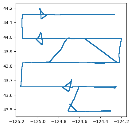
Now we can generate a simple map plot of the point GeoDataFrame

gdf_gps.plot(markersize=0.5)

<Axes: >

Slice and plot echo data based on selected ship track segments

Read all MVBS Zarr stores as a single dataset

Here we use the Xarray open_mfdataset function again to read all MVBS Zarr stores as a single dataset:

%%time
ds_MVBS = xr.open_mfdataset(
    str(MVBS_zarr_path / '*_MVBS.zarr'), 
    data_vars='minimal', coords='minimal',
    combine='by_coords',
    engine="zarr",
)

CPU times: user 2.43 s, sys: 68.9 ms, total: 2.49 s
Wall time: 2.48 s

Replace the channel dimension and coordinate with the frequency_nominal variable containing actual frequency values. Note that this step is possible only because there are no duplicated frequencies present.

ds_MVBS = ep.consolidate.swap_dims_channel_frequency(ds_MVBS)
ds_MVBS

<xarray.Dataset> Size: 32MB
Dimensions:            (frequency_nominal: 3, ping_time: 8649, depth: 152)
Coordinates:
  * frequency_nominal  (frequency_nominal) float64 24B 1.8e+04 3.8e+04 1.2e+05
  * depth              (depth) float64 1kB 0.0 5.0 10.0 ... 745.0 750.0 755.0
  * ping_time          (ping_time) datetime64[ns] 69kB 2017-07-28T00:05:20 .....
Data variables:
    Sv                 (frequency_nominal, ping_time, depth) float64 32MB dask.array<chunksize=(3, 59, 152), meta=np.ndarray>
    channel            (frequency_nominal) <U37 444B 'GPT  18 kHz 009072058c8...
Attributes:
    processing_function:          commongrid.compute_MVBS
    processing_software_name:     echopype
    processing_software_version:  0.9.0
    processing_time:              2024-08-08T20:28:04Z

xarray.Dataset

• Dimensions:
  • frequency_nominal: 3
  • ping_time: 8649
  • depth: 152
• Coordinates: (3)
  • frequency_nominal
    (frequency_nominal)
    float64
    1.8e+04 3.8e+04 1.2e+05

    long_name :

    Transducer frequency

    standard_name :

    sound_frequency

    units :

    Hz

    valid_min :

    0.0

    array([ 18000.,  38000., 120000.])

  • depth
    (depth)
    float64
    0.0 5.0 10.0 ... 745.0 750.0 755.0

    long_name :

    Range distance

    units :

    m

    array([  0.,   5.,  10.,  15.,  20.,  25.,  30.,  35.,  40.,  45.,  50.,  55.,
            60.,  65.,  70.,  75.,  80.,  85.,  90.,  95., 100., 105., 110., 115.,
           120., 125., 130., 135., 140., 145., 150., 155., 160., 165., 170., 175.,
           180., 185., 190., 195., 200., 205., 210., 215., 220., 225., 230., 235.,
           240., 245., 250., 255., 260., 265., 270., 275., 280., 285., 290., 295.,
           300., 305., 310., 315., 320., 325., 330., 335., 340., 345., 350., 355.,
           360., 365., 370., 375., 380., 385., 390., 395., 400., 405., 410., 415.,
           420., 425., 430., 435., 440., 445., 450., 455., 460., 465., 470., 475.,
           480., 485., 490., 495., 500., 505., 510., 515., 520., 525., 530., 535.,
           540., 545., 550., 555., 560., 565., 570., 575., 580., 585., 590., 595.,
           600., 605., 610., 615., 620., 625., 630., 635., 640., 645., 650., 655.,
           660., 665., 670., 675., 680., 685., 690., 695., 700., 705., 710., 715.,
           720., 725., 730., 735., 740., 745., 750., 755.])

  • ping_time
    (ping_time)
    datetime64[ns]
    2017-07-28T00:05:20 ... 2017-07-...

    axis :

    T

    long_name :

    Ping time

    standard_name :

    time

    array(['2017-07-28T00:05:20.000000000', '2017-07-28T00:05:40.000000000',
           '2017-07-28T00:06:00.000000000', ..., '2017-07-30T00:16:40.000000000',
           '2017-07-30T00:17:00.000000000', '2017-07-30T00:17:20.000000000'],
          dtype='datetime64[ns]')

• Data variables: (2)
  • Sv
    (frequency_nominal, ping_time, depth)
    float64
    dask.array<chunksize=(3, 59, 152), meta=np.ndarray>

    actual_range :

    [-98.73, 9.12]

    binning_mode :

    physical units

    cell_methods :

    ping_time: mean (interval: 20 second comment: ping_time is the interval start) depth: mean (interval: 5.0 meter comment: depth is the interval start)

    long_name :

    Mean volume backscattering strength (MVBS, mean Sv re 1 m-1)

    ping_time_interval :

    20s

    range_meter_interval :

    5.0m

    units :

    dB

    Array Chunk Bytes 30.09 MiB 363.38 kiB Shape (3, 8649, 152) (3, 102, 152) Dask graph 170 chunks in 341 graph layers Data type float64 numpy.ndarray

  • channel
    (frequency_nominal)
    <U37
    'GPT 18 kHz 009072058c8d 1-1 ES...

    long_name :

    Vendor channel ID

    array(['GPT  18 kHz 009072058c8d 1-1 ES18-11',
           'GPT  38 kHz 009072058146 2-1 ES38B',
           'GPT 120 kHz 00907205a6d0 4-1 ES120-7C'], dtype='<U37')

• Indexes: (3)
  • frequency_nominal
    PandasIndex

    PandasIndex(Index([18000.0, 38000.0, 120000.0], dtype='float64', name='frequency_nominal'))

  • depth
    PandasIndex

    PandasIndex(Index([  0.0,   5.0,  10.0,  15.0,  20.0,  25.0,  30.0,  35.0,  40.0,  45.0,
           ...
           710.0, 715.0, 720.0, 725.0, 730.0, 735.0, 740.0, 745.0, 750.0, 755.0],
          dtype='float64', name='depth', length=152))

  • ping_time
    PandasIndex

    PandasIndex(DatetimeIndex(['2017-07-28 00:05:20', '2017-07-28 00:05:40',
                   '2017-07-28 00:06:00', '2017-07-28 00:06:20',
                   '2017-07-28 00:06:40', '2017-07-28 00:07:00',
                   '2017-07-28 00:07:20', '2017-07-28 00:07:40',
                   '2017-07-28 00:08:00', '2017-07-28 00:08:20',
                   ...
                   '2017-07-30 00:14:20', '2017-07-30 00:14:40',
                   '2017-07-30 00:15:00', '2017-07-30 00:15:20',
                   '2017-07-30 00:15:40', '2017-07-30 00:16:00',
                   '2017-07-30 00:16:20', '2017-07-30 00:16:40',
                   '2017-07-30 00:17:00', '2017-07-30 00:17:20'],
                  dtype='datetime64[ns]', name='ping_time', length=8649, freq=None))

• Attributes: (4)

  processing_function :

  commongrid.compute_MVBS

  processing_software_name :

  echopype

  processing_software_version :

  0.9.0

  processing_time :

  2024-08-08T20:28:04Z

Extract MVBS along two N-S tracks

Below, we define two rectangular bounding boxes to extract two North-South-oriented ship track segments, then plot all GPS locations (red) and the bounding boxes (black) on a map.

We also plot the location of an Ocean Observatories Initiative (OOI) mooring (yellow star) from which the echosounder data is used in the OOI eclipse notebook in this repository.

More information on OOI can be found here: OOI.

tracksouth_bbox = gpd.GeoSeries(box(-125.17, 43.65, -125.14, 43.84), crs=gdf_gps.crs)
tracknorth_bbox = gpd.GeoSeries(box(-125.17, 43.98, -125.14, 44.17), crs=gdf_gps.crs)

basemap = cimgt.OSM()

_, ax = plt.subplots(
    figsize=(9, 7), subplot_kw={"projection": basemap.crs}
)
bnd = gdf_gps.geometry.bounds
ax.set_extent([bnd.minx.min() - 1, bnd.maxx.max() + 2, 
               bnd.miny.min() - 0.8, bnd.maxy.max() + 2.2])
ax.add_image(basemap, 7)
ax.gridlines(draw_labels=True, xformatter=LONGITUDE_FORMATTER, yformatter=LATITUDE_FORMATTER)

# GPS points
gdf_gps.plot(ax=ax, markersize=0.1, color='red', 
             transform=ccrs.PlateCarree())

# Bounding box for selected tracks
tracksouth_bbox.plot(ax=ax, edgecolor="black", linewidth=0.5, facecolor='none', 
                     transform=ccrs.PlateCarree())
tracknorth_bbox.plot(ax=ax, edgecolor="black", linewidth=0.5, facecolor='none', 
                     transform=ccrs.PlateCarree())

# OOI CE04 Oregon Offshore mooring location
plt.plot(-124.95, 44.37, marker='*', color='yellow', markersize=13, 
         transform=ccrs.PlateCarree());

Now we can clip the GeoDataFrame using the bounding boxes to extract the timestamps of the two North-South ship track segments (along the time1 coordinate), then use these timestamps to slice out MVBS datasets corresponding to these two ship track segments (along the ping_time coordinate).

This demonstrates the power of “label-aware” data selection and computation offered by Xarray, compared to pure NumPy implementations that require explicit indexing along the array dimensions.

gdf_gps_south = gpd.clip(gdf_gps, tracksouth_bbox)
ds_MVBS_south = ds_MVBS.sel(
    ping_time=slice(gdf_gps_south.index.min(), gdf_gps_south.index.max())
)

gdf_gps_north = gpd.clip(gdf_gps, tracknorth_bbox)
ds_MVBS_north = ds_MVBS.sel(
    ping_time=slice(gdf_gps_north.index.min(), gdf_gps_north.index.max())
)

Plot MVBS echograms for the two N-S tracks for all frequencies

Lastly, let’s plot the echogram along both ship track segments for all frequencies.

freq_len = ds_MVBS["frequency_nominal"].size

fig, ax = plt.subplots(freq_len, 2, constrained_layout=True, figsize=(12, 12))

for col_idx in range(2):  # left: south track, right: north track
    for freq_idx in range(freq_len):  # all frequencies
        axx = ax[freq_idx, col_idx]
        ds = ds_MVBS_south if col_idx == 0 else ds_MVBS_north
        ds["depth"].attrs["long_name"] = "Depth"
        (
            ds["Sv"]
            .isel(frequency_nominal=freq_idx)
            .plot(
                ax=axx,
                x='ping_time',
                y='depth',
                yincrease=False,
                vmin=-80, vmax=-50,
            )
        )
        if freq_idx < freq_len-1:
            axx.set_xlabel(None)

# Make titles for the two columns
ax[0, 0].text(
    0.5, 1.1, "South Track", ha="center", fontsize=16, fontweight="bold",
    transform=ax[0, 0].transAxes,  # use the axis coordinate
)
ax[0, 1].text(
    0.5, 1.1, "North Track", ha="center", fontsize=16, fontweight="bold",
    transform=ax[0, 1].transAxes,  # use the axis coordinate
)

plt.show()

Package versions

import datetime, s3fs
print(f"echopype: {ep.__version__}, xarray: {xr.__version__}, geopandas: {gpd.__version__}, "
      f"fsspec: {fsspec.__version__}, s3fs: {s3fs.__version__}")

print(f"\n{datetime.datetime.utcnow()} +00:00")

echopype: 0.9.0, xarray: 2024.6.0, geopandas: 1.0.1, fsspec: 2024.6.0, s3fs: 2024.6.0

2024-08-08 20:36:39.378317 +00:00