
Seafloor detection#
This notebook demonstrates how to:
Load and preprocess echosounder data using echopype
Detect the seafloor using two methods with detect_seafloor (basic thresholding and the Blackwell method)
Export and visualise the detected bottom line with echoregions
Apply the seafloor mask to the Sv data using apply_mask
Compute and visualise the mean volume backscattering strength (MVBS) from the masked data
First, we download the acoustic data.
import echopype as ep

raw_path = "s3://noaa-wcsd-pds/data/raw/Bell_M._Shimada/SH2306/EK80/Hake-D20230811-T165727.raw"
ed = ep.open_raw(
    raw_path,
    sonar_model="EK80",
    storage_options={"anon": True},
)
type(ed)
echopype.echodata.echodata.EchoData
We compute Sv and add transducer depth.
# Use the correct waveform_mode and encode_mode combination
ds_Sv = ep.calibrate.compute_Sv(ed, waveform_mode="CW", encode_mode="power")

# depth_offset=9.8 because transducer was on a lowered centerboard at 9.8 m deep
ds_Sv = ep.consolidate.add_depth(ds_Sv, ed, depth_offset=9.8)
We print the channel names.
channel_names = ds_Sv['channel'].values
channel_names
array(['WBT 400140-15 ES120-7C_ES', 'WBT 400141-15 ES18_ES',
       'WBT 400142-15 ES70-7C_ES', 'WBT 400143-15 ES38B_ES',
       'WBT 400145-15 ES200-7C_ES'], dtype=object)
We plot the raw Sv data.
ds_Sv["Sv"].plot(
    x="ping_time",
    row="channel", col_wrap=3,
    vmin=-80, vmax=-40,
    cmap="RdYlBu_r", yincrease=False
)
<xarray.plot.facetgrid.FacetGrid at 0x156200cfbf0>
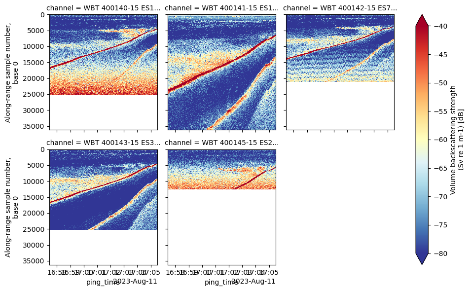
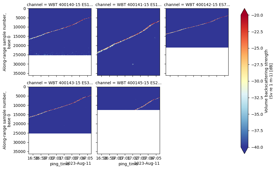
Adjust the colourbar range to highlight the seafloor.
ds_Sv["Sv"].plot(
    x="ping_time",
    row="channel", col_wrap=3,
    vmin=-40, vmax=-20,
    cmap="RdYlBu_r", yincrease=False
)
<xarray.plot.facetgrid.FacetGrid at 0x15623ac2600>
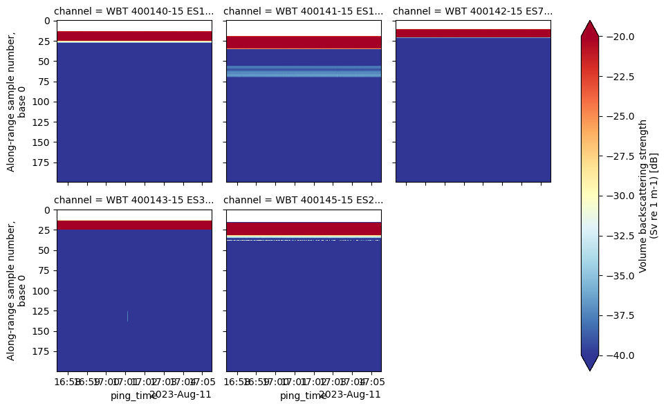
We show the 200 first samples, to observe the surface saturation zone. (We need to skip them to use the basic seafloor detection.)
ds_Sv.isel(range_sample=slice(0, 200))["Sv"].plot(
    x="ping_time",
    row="channel",
    col_wrap=3,
    vmin=-40, vmax=-20,
    cmap="RdYlBu_r",
    yincrease=False
)
<xarray.plot.facetgrid.FacetGrid at 0x15623f965a0>
We detect seafloor with the mask subpackage#
We use the basic bottom detection function from the seafloor_detection submodule within the echopype.mask package. We use here the 70 kHz channel to detect the seafloor.
sel_channel = "WBT 400142-15 ES70-7C_ES"

from echopype.mask import detect_seafloor
import xarray as xr

# Call detect_seafloor dispatcher
basic_depth = detect_seafloor(
    ds_Sv,
    method="basic",
    params={
        "var_name": "Sv",
        "channel": sel_channel,
        "threshold": (-40, -20),
        "offset_m": 0.5,
        "bin_skip_from_surface": 200, # due to surface saturation
    },
)

# Check output
assert isinstance(basic_depth, xr.DataArray)
assert set(basic_depth.dims) == {"ping_time"}
basic_depth
<xarray.DataArray 'bottom_depth' (ping_time: 213)> Size: 2kB
array([496.54757004, 495.62407996, 492.99568514, 490.75799766,
       488.80446096, 486.95748082, 486.03399074, 485.03946297,
       483.44111477, 481.52309693, 479.42748484, 478.18432512,
       475.98215649, 473.63791246, 471.61333807, 469.76635792,
       468.48767936, 467.38659504, 465.93032223, 464.36749288,
       462.87570122, 461.59702266, 459.60796712, 457.29924194,
       455.27466754, 452.11348999, 450.87033027, 447.88674696,
       445.47146523, 443.76656048, 441.81302379, 439.39774206,
       437.16005457, 435.13548018, 434.03439587, 431.58359529,
       429.80765284, 429.09727586, 426.29128679, 423.76944852,
       420.67930866, 419.0454416 , 416.13289599, 413.68209541,
       410.91162519, 408.8870508 , 406.68488217, 404.26960044,
       401.67672446, 400.2559705 , 398.62210345, 396.63304791,
       394.92814316, 393.15220071, 390.77243783, 388.92545769,
       387.14951524, 386.29706286, 384.76975236, 382.49654602,
       381.14682976, 379.90367005, 378.16324645, 376.10315321,
       374.54032386, 372.9774945 , 371.76985364, 369.7807981 ,
       367.9693368 , 365.76716816, 364.73712154, 363.95570687,
       362.92566025, 361.54042514, 359.69344499, 358.30820988,
       356.99401247, 355.43118312, 353.51316527, 352.02137362,
...
       274.41268864, 273.09849123, 271.74877497, 269.97283252,
       268.41000316, 266.88269266, 265.28434446, 262.94010042,
       261.23519567, 260.20514905, 258.81991395, 256.8308584 ,
       254.20246358, 251.57406876, 250.04675825, 247.88010847,
       245.67793983, 243.79544084, 241.27360256, 239.24902817,
       236.86926529, 234.16983277, 232.00318298, 229.83653319,
       227.38573262, 226.00049751, 223.51417808, 221.41856599,
       218.86120887, 216.65904023, 214.52790929, 212.5033349 ,
       210.51427936, 208.95145001, 206.67824367, 204.12088655,
       202.2028687 , 199.64551158, 197.79853143, 196.23570208,
       194.38872193, 192.29310984, 190.2330166 , 188.42155531,
       186.92976365, 184.58551962, 183.02269026, 181.31778551,
       179.08009803, 177.37519328, 175.45717544, 173.64571414,
       171.86977169, 170.59109313, 169.34793341, 169.06378262,
       168.92170723, 168.88618838, 168.2468491 , 167.71406636,
       167.00368938, 166.47090665, 165.33430348, 163.06109715,
       161.46274895, 160.61029657, 159.5447311 , 157.9463829 ,
       155.35350692, 152.54751786, 149.84808534, 148.28525598,
       146.86450202, 145.37271037, 144.73337109, 144.52025799,
       144.12955065])
Coordinates:
  * ping_time  (ping_time) datetime64[ns] 2kB 2023-08-11T16:57:27.277163 ... ...
Attributes:
    detector:               basic
    threshold_min:          -40.0
    threshold_max:          -20.0
    offset_m:               0.5
    bin_skip_from_surface:  200
channel: WBT 400142-15 ES70-7C_ESprint(type(basic_depth)) # should be xarray.DataArray
basic_depth.coords
<class 'xarray.core.dataarray.DataArray'>
Coordinates:
* ping_time (ping_time) datetime64[ns] 2kB 2023-08-11T16:57:27.277163 ... ...
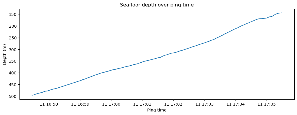
We plot the seafloor. The bottom is computed because we access it.
import matplotlib.pyplot as plt
fig, ax = plt.subplots(figsize=(12, 4))
ax.plot(basic_depth["ping_time"].values, basic_depth.values, fillstyle='full', markersize=1)
ax.set_title("Seafloor depth over ping time")
ax.set_xlabel("Ping time")
ax.set_ylabel("Depth (m)")
ax.invert_yaxis()
plt.show()
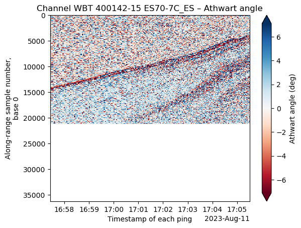
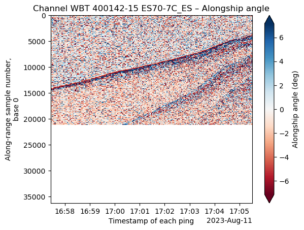
We compare the results with the Blackwell method, which requires the angle_alongship and angle_athwartship variables.
# Add split-beam angles
ds_Sv = ep.consolidate.add_splitbeam_angle(
ds_Sv,
ed,
waveform_mode="CW",
encode_mode="power",
to_disk=False,
)
required_vars = ["Sv", "angle_alongship", "angle_athwartship", "depth"]
missing = [var for var in required_vars if var not in ds_Sv]
if not missing:
print("All required variables are present for Blackwell detection.")
else:
print(f"Missing required variables: {missing}.")
All required variables are present for Blackwell detection.
import matplotlib.pyplot as plt
ds_Sv["angle_athwartship"].sel(channel=sel_channel).plot(
x="ping_time",
y="range_sample",
cmap="RdBu",
yincrease=False,
robust=True,
cbar_kwargs={"label": "Athwart angle (deg)"}
)
plt.title(f"Channel {sel_channel} – Athwart angle")
plt.show()
ds_Sv["angle_alongship"].sel(channel=sel_channel).plot(
x="ping_time",
y="range_sample",
cmap="RdBu",
yincrease=False,
robust=True,
cbar_kwargs={"label": "Alongship angle (deg)"}
)
plt.title(f"Channel {sel_channel} – Alongship angle")
plt.show()
We run the Blackwell seafloor detection.
blackwell_depth = detect_seafloor(
ds=ds_Sv,
method="blackwell",
params={
"channel": sel_channel,
"var_name": "Sv",
"threshold": [-40, 2.4, 1.0],
"offset": 0.5,
"r0": 10,
"r1": 1000,
"wtheta": 28,
"wphi": 52,
}
)
# Check output
assert isinstance(blackwell_depth, xr.DataArray)
assert set(blackwell_depth.dims) == {"ping_time"}
blackwell_depth
<xarray.DataArray 'bottom_depth' (ping_time: 213)> Size: 2kB
array([496.54757004, 495.62407996, 492.99568514, 490.75799766,
488.80446096, 486.95748082, 486.03399074, 485.03946297,
483.44111477, 481.52309693, 479.42748484, 478.18432512,
475.98215649, 473.63791246, 471.61333807, 469.76635792,
468.48767936, 467.38659504, 465.93032223, 464.36749288,
462.87570122, 461.59702266, 459.60796712, 457.29924194,
455.27466754, 452.11348999, 450.87033027, 447.88674696,
445.47146523, 443.76656048, 441.81302379, 439.39774206,
437.16005457, 435.13548018, 434.03439587, 431.58359529,
429.80765284, 429.09727586, 426.29128679, 423.76944852,
420.67930866, 419.0454416 , 416.13289599, 413.68209541,
410.91162519, 408.8870508 , 406.68488217, 404.26960044,
401.67672446, 400.2559705 , 398.62210345, 396.63304791,
394.92814316, 393.15220071, 390.77243783, 388.92545769,
387.14951524, 386.29706286, 384.76975236, 382.49654602,
381.14682976, 379.90367005, 378.16324645, 376.10315321,
374.54032386, 372.9774945 , 371.76985364, 369.7807981 ,
367.9693368 , 365.76716816, 364.73712154, 363.95570687,
362.92566025, 361.54042514, 359.69344499, 358.30820988,
356.99401247, 355.43118312, 353.51316527, 352.02137362,
...
274.41268864, 273.09849123, 271.74877497, 269.97283252,
268.41000316, 266.88269266, 265.28434446, 262.94010042,
261.23519567, 260.20514905, 258.81991395, 256.8308584 ,
254.20246358, 251.57406876, 250.04675825, 247.88010847,
245.67793983, 243.79544084, 241.27360256, 239.24902817,
236.86926529, 234.16983277, 232.00318298, 229.83653319,
227.38573262, 226.00049751, 223.51417808, 221.41856599,
218.86120887, 216.65904023, 214.52790929, 212.5033349 ,
210.51427936, 208.95145001, 206.67824367, 204.12088655,
202.2028687 , 199.64551158, 197.79853143, 196.23570208,
194.38872193, 192.29310984, 190.2330166 , 188.42155531,
186.92976365, 184.58551962, 183.02269026, 181.31778551,
179.08009803, 177.37519328, 175.45717544, 173.64571414,
171.86977169, 170.59109313, 169.34793341, 169.06378262,
168.92170723, 168.88618838, 168.2468491 , 167.71406636,
167.00368938, 166.47090665, 165.33430348, 163.06109715,
161.46274895, 160.61029657, 159.5447311 , 157.9463829 ,
155.35350692, 152.54751786, 149.84808534, 148.28525598,
146.86450202, 145.37271037, 144.73337109, 144.52025799,
144.3071449 ])
Coordinates:
* ping_time (ping_time) datetime64[ns] 2kB 2023-08-11T16:57:27.277163 ... ...
Attributes:
detector: blackwell
threshold_Sv: -40.0
threshold_angle_major: 2.4
threshold_angle_minor: 1.0
offset_m: 0.5
channel: WBT 400142-15 ES70-7C_ESWe compare the results from both seafloor detection methods.
# Get the ping_time values from each DataArray
pt_basic = basic_depth.ping_time
pt_blackwell = blackwell_depth.ping_time
# Find ping times in basic_depth but not in blackwell_depth
missing_in_blackwell = pt_basic[~pt_basic.isin(pt_blackwell)]
print(f"Ping times in basic_depth but missing in blackwell_depth: {missing_in_blackwell.size}")
print(missing_in_blackwell.values)
# Find ping times in blackwell_depth but not in basic_depth
missing_in_basic = pt_blackwell[~pt_blackwell.isin(pt_basic)]
print(f"Ping times in blackwell_depth but missing in basic_depth: {missing_in_basic.size}")
print(missing_in_basic.values)
Ping times in basic_depth but missing in blackwell_depth: 0
[]
Ping times in blackwell_depth but missing in basic_depth: 0
[]
print("bd.ping_time:", basic_depth)#.ping_time)
print("\n\n")
print("bw.ping_time:", blackwell_depth)#.ping_time)
bd.ping_time: <xarray.DataArray 'bottom_depth' (ping_time: 213)> Size: 2kB
array([496.54757004, 495.62407996, 492.99568514, 490.75799766,
       488.80446096, 486.95748082, 486.03399074, 485.03946297,
       483.44111477, 481.52309693, 479.42748484, 478.18432512,
       475.98215649, 473.63791246, 471.61333807, 469.76635792,
       468.48767936, 467.38659504, 465.93032223, 464.36749288,
       462.87570122, 461.59702266, 459.60796712, 457.29924194,
       455.27466754, 452.11348999, 450.87033027, 447.88674696,
       445.47146523, 443.76656048, 441.81302379, 439.39774206,
       437.16005457, 435.13548018, 434.03439587, 431.58359529,
       429.80765284, 429.09727586, 426.29128679, 423.76944852,
       420.67930866, 419.0454416 , 416.13289599, 413.68209541,
       410.91162519, 408.8870508 , 406.68488217, 404.26960044,
       401.67672446, 400.2559705 , 398.62210345, 396.63304791,
       394.92814316, 393.15220071, 390.77243783, 388.92545769,
       387.14951524, 386.29706286, 384.76975236, 382.49654602,
       381.14682976, 379.90367005, 378.16324645, 376.10315321,
       374.54032386, 372.9774945 , 371.76985364, 369.7807981 ,
       367.9693368 , 365.76716816, 364.73712154, 363.95570687,
       362.92566025, 361.54042514, 359.69344499, 358.30820988,
       356.99401247, 355.43118312, 353.51316527, 352.02137362,
...
       274.41268864, 273.09849123, 271.74877497, 269.97283252,
       268.41000316, 266.88269266, 265.28434446, 262.94010042,
       261.23519567, 260.20514905, 258.81991395, 256.8308584 ,
       254.20246358, 251.57406876, 250.04675825, 247.88010847,
       245.67793983, 243.79544084, 241.27360256, 239.24902817,
       236.86926529, 234.16983277, 232.00318298, 229.83653319,
       227.38573262, 226.00049751, 223.51417808, 221.41856599,
       218.86120887, 216.65904023, 214.52790929, 212.5033349 ,
       210.51427936, 208.95145001, 206.67824367, 204.12088655,
       202.2028687 , 199.64551158, 197.79853143, 196.23570208,
       194.38872193, 192.29310984, 190.2330166 , 188.42155531,
       186.92976365, 184.58551962, 183.02269026, 181.31778551,
       179.08009803, 177.37519328, 175.45717544, 173.64571414,
       171.86977169, 170.59109313, 169.34793341, 169.06378262,
       168.92170723, 168.88618838, 168.2468491 , 167.71406636,
       167.00368938, 166.47090665, 165.33430348, 163.06109715,
       161.46274895, 160.61029657, 159.5447311 , 157.9463829 ,
       155.35350692, 152.54751786, 149.84808534, 148.28525598,
       146.86450202, 145.37271037, 144.73337109, 144.52025799,
       144.12955065])
Coordinates:
  * ping_time  (ping_time) datetime64[ns] 2kB 2023-08-11T16:57:27.277163 ... ...
Attributes:
detector: basic
threshold_min: -40.0
threshold_max: -20.0
offset_m: 0.5
bin_skip_from_surface: 200
channel: WBT 400142-15 ES70-7C_ES
bw.ping_time: <xarray.DataArray 'bottom_depth' (ping_time: 213)> Size: 2kB
array([496.54757004, 495.62407996, 492.99568514, 490.75799766,
       488.80446096, 486.95748082, 486.03399074, 485.03946297,
       483.44111477, 481.52309693, 479.42748484, 478.18432512,
       475.98215649, 473.63791246, 471.61333807, 469.76635792,
       468.48767936, 467.38659504, 465.93032223, 464.36749288,
       462.87570122, 461.59702266, 459.60796712, 457.29924194,
       455.27466754, 452.11348999, 450.87033027, 447.88674696,
       445.47146523, 443.76656048, 441.81302379, 439.39774206,
       437.16005457, 435.13548018, 434.03439587, 431.58359529,
       429.80765284, 429.09727586, 426.29128679, 423.76944852,
       420.67930866, 419.0454416 , 416.13289599, 413.68209541,
       410.91162519, 408.8870508 , 406.68488217, 404.26960044,
       401.67672446, 400.2559705 , 398.62210345, 396.63304791,
       394.92814316, 393.15220071, 390.77243783, 388.92545769,
       387.14951524, 386.29706286, 384.76975236, 382.49654602,
       381.14682976, 379.90367005, 378.16324645, 376.10315321,
       374.54032386, 372.9774945 , 371.76985364, 369.7807981 ,
       367.9693368 , 365.76716816, 364.73712154, 363.95570687,
       362.92566025, 361.54042514, 359.69344499, 358.30820988,
       356.99401247, 355.43118312, 353.51316527, 352.02137362,
...
       274.41268864, 273.09849123, 271.74877497, 269.97283252,
       268.41000316, 266.88269266, 265.28434446, 262.94010042,
       261.23519567, 260.20514905, 258.81991395, 256.8308584 ,
       254.20246358, 251.57406876, 250.04675825, 247.88010847,
       245.67793983, 243.79544084, 241.27360256, 239.24902817,
       236.86926529, 234.16983277, 232.00318298, 229.83653319,
       227.38573262, 226.00049751, 223.51417808, 221.41856599,
       218.86120887, 216.65904023, 214.52790929, 212.5033349 ,
       210.51427936, 208.95145001, 206.67824367, 204.12088655,
       202.2028687 , 199.64551158, 197.79853143, 196.23570208,
       194.38872193, 192.29310984, 190.2330166 , 188.42155531,
       186.92976365, 184.58551962, 183.02269026, 181.31778551,
       179.08009803, 177.37519328, 175.45717544, 173.64571414,
       171.86977169, 170.59109313, 169.34793341, 169.06378262,
       168.92170723, 168.88618838, 168.2468491 , 167.71406636,
       167.00368938, 166.47090665, 165.33430348, 163.06109715,
       161.46274895, 160.61029657, 159.5447311 , 157.9463829 ,
       155.35350692, 152.54751786, 149.84808534, 148.28525598,
       146.86450202, 145.37271037, 144.73337109, 144.52025799,
       144.3071449 ])
Coordinates:
* ping_time (ping_time) datetime64[ns] 2kB 2023-08-11T16:57:27.277163 ... ...
Attributes:
detector: blackwell
threshold_Sv: -40.0
threshold_angle_major: 2.4
threshold_angle_minor: 1.0
offset_m: 0.5
channel: WBT 400142-15 ES70-7C_ES
# Align both bottom detections on ping_time using xarray
bd, bw = xr.align(basic_depth, blackwell_depth, join="inner")
assert bd.ping_time.equals(bw.ping_time), "Ping times are not aligned."

# Compute difference
diff = bd - bw
common_time = bd.ping_time  # aligned time axis, pick any

# plot
fig, axs = plt.subplots(nrows=1, ncols=2, figsize=(14, 5), sharex=True)

# p1: depth from both methods
axs[0].plot(common_time, bd, label="Basic", color="navy")
axs[0].plot(common_time, bw, label="Blackwell", color="firebrick", linestyle="--")
axs[0].invert_yaxis()
axs[0].set_title("Seafloor depth over ping time")
axs[0].set_xlabel("Ping time")
axs[0].set_ylabel("Depth (m)")
axs[0].legend()
axs[0].grid(True)

# p2: difference
axs[1].plot(common_time, diff, color="darkgreen")
axs[1].axhline(0, color="gray", linestyle="--", linewidth=1)
axs[1].set_title("Difference: Basic – Blackwell")
axs[1].set_xlabel("Ping time")
axs[1].set_ylabel("Depth difference (m)")
axs[1].grid(True)

plt.tight_layout()
plt.show()
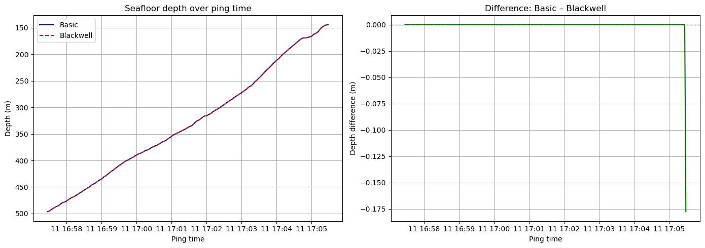
# Show last 10 values of each
print("Last 10 bottom_depth values (Basic):")
print(bd.values[-10:])

print("\nLast 10 blackwell_bottom values (Blackwell):")
print(bw.values[-10:])
Last 10 bottom_depth values (Basic):
[157.9463829  155.35350692 152.54751786 149.84808534 148.28525598
 146.86450202 145.37271037 144.73337109 144.52025799 144.12955065]

Last 10 blackwell_bottom values (Blackwell):
[157.9463829  155.35350692 152.54751786 149.84808534 148.28525598
 146.86450202 145.37271037 144.73337109 144.52025799 144.3071449 ]
Next, we aim to mask the seafloor in ds_Sv.
The echoregions package expects an xarray.DataArray as input, with depth provided. However, in raw Sv datasets like ds_Sv, depth is typically stored as a data variable, not a coordinate. As a result, directly passing ds_Sv[“Sv”] to lines() does not work, because the depth information is not attached to the Sv DataArray.
As a temporary workaround, we create a new Dataset (ds_single) where depth is explicitly defined as a coordinate. This allows Sv to be treated as a proper 2D DataArray over (ping_time, depth) for a single channel, as required by echoregions for bottom masking and region selection.
import xarray as xr

selected_channel = "WBT 400141-15 ES18_ES"
frequency_dict = {
    "WBT 400140-15 ES120-7C_ES": 120000,
    "WBT 400141-15 ES18_ES": 18000,
    "WBT 400142-15 ES70-7C_ES": 70000,
    "WBT 400143-15 ES38B_ES": 38000,
    "WBT 400145-15 ES200-7C_ES": 200000,
}

# Extract Sv, time, and depth (first ping)
Sv_da = ds_Sv["Sv"].sel(channel=selected_channel)
depth = ds_Sv["depth"].sel(channel=selected_channel).isel(ping_time=0)

# Build DataArray with (ping_time, depth) and add channel dim
Sv_plot = xr.DataArray(
    data=Sv_da.values,
    dims=["ping_time", "depth"],
    coords={"ping_time": Sv_da["ping_time"], "depth": depth.data},
    name="Sv"
).expand_dims(channel=[selected_channel])

# Wrap into Dataset and add frequency_nominal
ds_single = xr.Dataset({
    "Sv": Sv_plot,
    "frequency_nominal": xr.DataArray([frequency_dict[selected_channel]], dims=["channel"], coords={"channel": [selected_channel]})
})
ds_single
<xarray.Dataset> Size: 62MB
Dimensions:            (channel: 1, ping_time: 213, depth: 36198)
Coordinates:
  * channel            (channel) object 8B 'WBT 400141-15 ES18_ES'
  * ping_time          (ping_time) datetime64[ns] 2kB 2023-08-11T16:57:27.277...
  * depth              (depth) float64 290kB 9.8 9.821 9.841 ... 759.8 759.8
Data variables:
    Sv                 (channel, ping_time, depth) float64 62MB nan ... -70.16
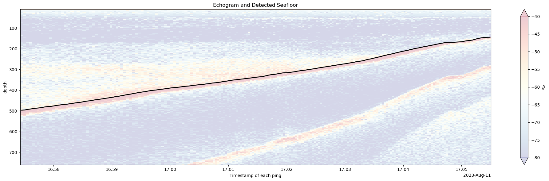
frequency_nominal (channel) int64 8B 18000We can now use echoregions to generate a mask from the detected seafloor line. (Note: the mask is applied here only to a single frequency.)
import pandas as pd

# Create minimal DataFrame with required columns
df = pd.DataFrame({
    "time": blackwell_depth["ping_time"].values,
    "depth": blackwell_depth.values,
})

# Save to CSV (required at the moment)
# For now commented, because already exist in ./example_data
# df.to_csv("./example_data/seafloor_detection/bottom_depth_minimal.csv", index=False)
import echoregions as er

lines = er.read_lines_csv("./example_data/seafloor_detection/bottom_depth_minimal.csv")
plt.figure(figsize=(20, 6))

# Plot Sv echogram for one channel
ds_single["Sv"].isel(channel=0).T.plot.pcolormesh(
    y="depth",
    cmap="RdYlBu_r",
    yincrease=False,
    vmin=-80,
    vmax=-40,
    alpha=0.2
)

# Plot seafloor line from echoregions Lines object
plt.plot(
    lines.data['time'], lines.data['depth'],
    color='black', label='Bottom', linewidth=2
)

plt.title("Echogram and Detected Seafloor")
plt.tight_layout()
plt.show()
# Use the built in mask function
bottom_mask_da, bottom_points = lines.seafloor_mask(
    ds_single.Sv, # Pass a DataArray where depth is a coordinate
    operation="above_below",
    method="slinear",
    limit_area=None,
    limit_direction="both"
)

bottom_mask_da
<xarray.DataArray (depth: 36198, ping_time: 213)> Size: 62MB
array([[0, 0, 0, ..., 0, 0, 0],
       [0, 0, 0, ..., 0, 0, 0],
       [0, 0, 0, ..., 0, 0, 0],
       ...,
       [1, 1, 1, ..., 1, 1, 1],
       [1, 1, 1, ..., 1, 1, 1],
       [1, 1, 1, ..., 1, 1, 1]], shape=(36198, 213))
Coordinates:
  * depth      (depth) float64 290kB 9.8 9.821 9.841 9.862 ... 759.7 759.8 759.8
* ping_time (ping_time) datetime64[ns] 2kB 2023-08-11T16:57:27.277163 ... ...import numpy as np
print("Unique Values in Bottom Mask:", np.unique(bottom_mask_da.data))
Unique Values in Bottom Mask: [0 1]
print("Bottom Mask Ping Time Dimension Length:", len(bottom_mask_da["ping_time"]))
print("Bottom Mask Depth Dimension Length:", len(bottom_mask_da["depth"]))
print("Echogram Ping Time Dimension Length:", len(ds_single.Sv["ping_time"]))
print("Echogram Depth Dimension Length:", len(ds_single.Sv["depth"]))
Bottom Mask Ping Time Dimension Length: 213
Bottom Mask Depth Dimension Length: 36198
Echogram Ping Time Dimension Length: 213
Echogram Depth Dimension Length: 36198
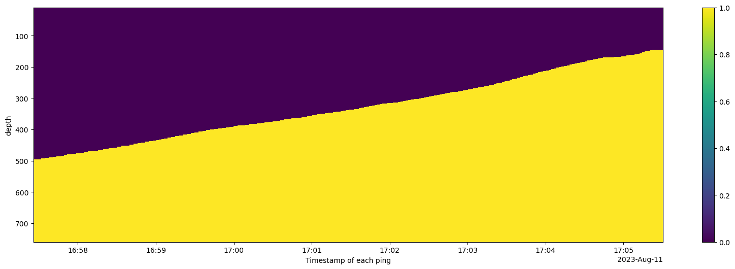
We plot the mask.
plt.figure(figsize = (20, 6))
bottom_mask_da.plot(y="depth", yincrease=False)
<matplotlib.collections.QuadMesh at 0x15624735a00>
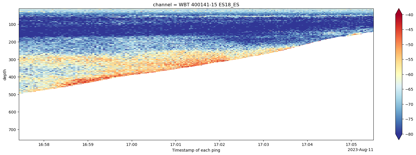
# Invert 1/0 or True/False mask to match echopype apply_mask expectations
inverted_mask = ~bottom_mask_da.astype(bool)
import echopype as ep

# Get only channel values where the mask is 1
mask_exists_Sv = xr.where(
    inverted_mask == 1,
    ds_single["Sv"].isel(channel=0),
    np.nan,
)

# Plot the masked Sv
plt.figure(figsize = (20, 6))
mask_exists_Sv.plot(y="depth", cmap="RdYlBu_r", yincrease=False, vmin=-80, vmax=-40)
<matplotlib.collections.QuadMesh at 0x15624719fa0>
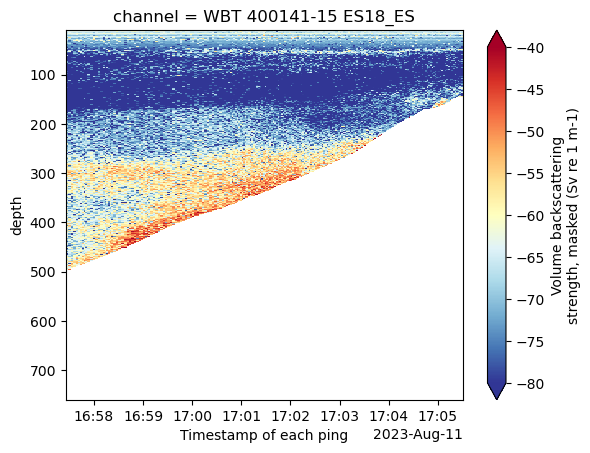
We use apply_mask from the echopype.mask to the dataset
from echopype.mask import apply_mask
import numpy as np

print(ds_single["Sv"].dims)
print(ds_single["Sv"].shape)
print(inverted_mask.dims)
print(inverted_mask.shape)

# Transpose to match ('ping_time', 'depth')
bottom_mask_fixed = inverted_mask.transpose("ping_time", "depth")

print(ds_single["Sv"].dims)
print(ds_single["Sv"].shape)
print(bottom_mask_fixed.dims)
print(bottom_mask_fixed.shape)

ds_with_mask = apply_mask(ds_single, bottom_mask_fixed, var_name="Sv", fill_value=np.nan)
('channel', 'ping_time', 'depth')
(1, 213, 36198)
('depth', 'ping_time')
(36198, 213)
('channel', 'ping_time', 'depth')
(1, 213, 36198)
('ping_time', 'depth')
(213, 36198)
ds_with_mask
<xarray.Dataset> Size: 62MB
Dimensions:            (channel: 1, ping_time: 213, depth: 36198)
Coordinates:
  * channel            (channel) object 8B 'WBT 400141-15 ES18_ES'
  * ping_time          (ping_time) datetime64[ns] 2kB 2023-08-11T16:57:27.277...
  * depth              (depth) float64 290kB 9.8 9.821 9.841 ... 759.8 759.8
Data variables:
    Sv                 (channel, ping_time, depth) float64 62MB nan nan ... nan
    frequency_nominal  (channel) int64 8B 18000
Attributes:
    mask_software_name:     echopype
    mask_software_version:  0.11.2.dev18+gf58dd2eb2.d20260429
    mask_time:              2026-05-07T02:15:34+00:00
mask_function: mask.apply_maskds_with_mask["Sv"].plot(
x="ping_time",
vmin=-80, vmax=-40,
cmap="RdYlBu_r", yincrease=False
)
<matplotlib.collections.QuadMesh at 0x1563f559130>
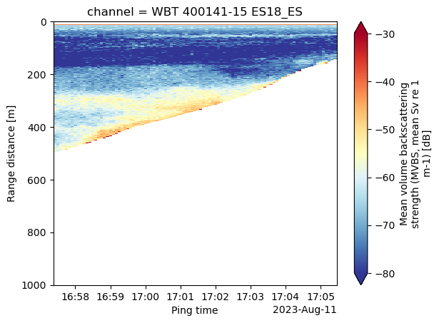
We compute and plot MVBS using the mask computed with the mask subpackage.
# Compute MVBS
ds_MVBS_mask = ep.commongrid.compute_MVBS(
    ds_with_mask,
    range_var="depth",
    range_bin="1m",
    ping_time_bin="5s",
    range_var_max="1000m",
)

ds_MVBS_mask["Sv"].plot(
    x="ping_time", cmap='RdYlBu_r', yincrease=False,
    vmin=-80, vmax=-30
)
<matplotlib.collections.QuadMesh at 0x1563efa2810>
from datetime import datetime, timezone
import dask

print(f"echopype: {ep.__version__}, dask: {dask.__version__}")
print(f"\n{datetime.now(timezone.utc)}")
echopype: 0.11.2.dev18+gf58dd2eb2.d20260429, dask: 2026.3.0

2026-05-07 02:15:38.870010+00:00