
Identify zooplankton school from glider echosounder data with external location and environmental data incorporated#
This notebook accompanies the following paper:
Echopype: Interoperable and scalable echosounder data processing with Echopype
Authors: Wu-Jung Lee, Landung Setiawan, Caesar Tuguinay, Emilio Mayorga, and Valentina Staneva
ICES Journal of Marine Science 2024: https://doi.org/10.1093/icesjms/fsae133
Introduction#
Description#
This notebook uses echosounder data from a glider to illustrate how Echopype can use external location (latitude and longitude) and environmental (temperature, salinity and pressure) data in the processing, if the data do not already exist in the echosounder raw files or if users would like to udpdate them. The data are provided by Delphine Mossman from the Department of Marine and Coastal Sciences at Rutgers University. The data were a 15-min section of echosounder data collected by an Acoustic Zooplankton and Fisher Profiler (AZFP) mounted on a Slocum glider deployed in the Southern Ocean off Antarctica (Ross Sea) in 2018.
In this notebook we attempt to correct for the glider orientation and identify zooplankton swarms in the echogram following steps detailed in the 2021 M.S. thesis from Ailey Sheehan, another member of the same Rutgers team. The computations are available in the associated GitHub repository.
Outline#
Running the notebook#
This notebook can be run with a conda environment created using the conda environment file. It uses data files found in the notebooks/example_data/glider_AZFP directory in this repository.
Note#
We encourage importing Echopype as ep for consistency.
from pathlib import Path

import geopandas as gpd
import pandas as pd
import xarray as xr
from scipy.spatial.transform import Rotation as R
import numpy as np

import matplotlib.pyplot as plt
import cartopy.crs as ccrs

import echopype as ep
import echopype.colormap

import warnings
warnings.simplefilter("ignore", category=DeprecationWarning)
Path setup#
# Set path to example data
data_path = Path('./example_data/glider_AZFP')
Data processing workflow#
Open and convert raw AZFP data#
To open an AZFP data file (*.01A files), the accompanying XML metadata file must be provided.
# Open RAW
azfp_data_fpath = data_path / "18011107.01A"
ed = ep.open_raw(
    azfp_data_fpath,
    xml_path=data_path / "18011107.XML",
    sonar_model="AZFP"
)
ed
-
<xarray.DatasetView> Size: 0B Dimensions: () Data variables: *empty* Attributes: conventions: CF-1.7, SONAR-netCDF4-1.0, ACDD-1.3 keywords: AZFP sonar_convention_authority: ICES sonar_convention_name: SONAR-netCDF4 sonar_convention_version: 1.0 summary: title: date_created: 2018-01-11T07:44:40Z -
<xarray.DatasetView> Size: 188B Dimensions: (channel: 3) Coordinates: * channel (channel) <U11 132B '59006-38-1' ... '59006-200-3' Data variables: absorption_indicative (channel) float64 24B nan nan nan sound_speed_indicative float64 8B nan frequency_nominal (channel) float64 24B 3.8e+04 1.25e+05 2e+05 -
<xarray.DatasetView> Size: 380B Dimensions: (time1: 1, time2: 1, channel: 3) Coordinates: * time1 (time1) datetime64[ns] 8B 2018-01-11T07:44:40 * time2 (time2) datetime64[ns] 8B 2018-01-11T07:44:40 * channel (channel) <U11 132B '59006-38-1' ... '59006-200-3' Data variables: (12/21) latitude (time1) float64 8B nan longitude (time1) float64 8B nan pitch (time2) float64 8B nan roll (time2) float64 8B nan vertical_offset (time2) float64 8B nan water_level float64 8B nan ... ... MRU_rotation_y float64 8B nan MRU_rotation_z float64 8B nan position_offset_x float64 8B nan position_offset_y float64 8B nan position_offset_z float64 8B nan frequency_nominal (channel) float64 24B 3.8e+04 1.25e+05 2e+05 Attributes: platform_name: platform_type: platform_code_ICES: -
<xarray.DatasetView> Size: 304B Dimensions: (filenames: 1) Coordinates: * filenames (filenames) int64 8B 0 Data variables: source_filenames (filenames) <U37 148B 'example_data/glider_AZFP/18... meta_source_filenames (filenames) <U37 148B 'example_data/glider_AZFP/18... Attributes: conversion_software_name: echopype conversion_software_version: 0.11.1 conversion_time: 2026-04-18T19:38:12+00:00 -
<xarray.DatasetView> Size: 372B Dimensions: (beam_group: 1) Coordinates: * beam_group (beam_group) <U11 44B 'Beam_group1' Data variables: beam_group_descr (beam_group) <U82 328B 'contains backscatter power (unc... Attributes: sonar_manufacturer: ASL Environmental Sciences sonar_model: AZFP sonar_serial_number: 59006 sonar_software_name: AZFP sonar_software_version: based on AZFP Matlab version 1.4 sonar_type: echosounder -
<xarray.DatasetView> Size: 22MB Dimensions: (channel: 3, ping_time: 920, range_sample: 1999, beam_group: 1) Coordinates: * channel (channel) <U11 132B '59006-38-1' ... '59006-... * ping_time (ping_time) datetime64[ns] 7kB 2018-01-11T07... * range_sample (range_sample) int64 16kB 0 1 2 ... 1997 1998 * beam_group (beam_group) <U11 44B 'Beam_group1' Data variables: (12/16) frequency_nominal (channel) float64 24B 3.8e+04 1.25e+05 2e+05 beam_type (channel) int64 24B 0 0 0 beam_direction_x (channel) float64 24B nan nan nan beam_direction_y (channel) float64 24B nan nan nan beam_direction_z (channel) float64 24B nan nan nan backscatter_r (channel, ping_time, range_sample) float32 22MB ... ... ... transmit_frequency_start (channel) float64 24B 3.8e+04 1.25e+05 2e+05 transmit_frequency_stop (channel) float64 24B 3.8e+04 1.25e+05 2e+05 transmit_type <U2 8B 'CW' beam_stabilisation int8 1B 0 non_quantitative_processing int16 2B 0 sample_time_offset float64 8B 0.0 Attributes: beam_mode: conversion_equation_t: type_4 -
<xarray.DatasetView> Size: 148kB
Dimensions:                                         (channel: 3,
                                                     ping_time: 920,
                                                     ancillary_len: 5,
                                                     ad_len: 2,
                                                     phase_number: 1, cpu: 0,
                                                     serial_number: 2,
                                                     XML_sonar_serial_number: 2)
Coordinates:
  * channel                                         (channel) <U11 132B '5900...
  * ping_time                                       (ping_time) datetime64[ns] 7kB ...
  * ancillary_len                                   (ancillary_len) int64 40B ...
  * ad_len                                          (ad_len) int64 16B 0 1
  * phase_number                                    (phase_number) int64 8B 1
  * cpu                                             (cpu) float64 0B
  * serial_number                                   (serial_number) int64 16B ...
  * XML_sonar_serial_number                         (XML_sonar_serial_number) int64 16B ...
Data variables: (12/71)
    frequency_nominal                               (channel) float64 24B 3.8...
    digitization_rate                               (channel) int64 24B 20000...
    lock_out_index                                  (channel) int64 24B 0 0 0
    number_of_bins_per_channel                      (channel) int64 24B 1999 ...
    number_of_samples_per_average_bin               (channel) int64 24B 1 1 1
    board_number                                    (channel) int64 24B 0 1 2
    ...                                              ...
    tilt_X_c                                        float64 8B 0.0
    tilt_X_d                                        float64 8B 0.0
    tilt_Y_a                                        float64 8B 0.0
    tilt_Y_b                                        float64 8B 0.0
    tilt_Y_c                                        float64 8B 0.0
    tilt_Y_d                                        float64 8B 0.0
AZFP raw data files doesn’t contain latitude longitude data. Therefore, the Platform group should have NaNs for this location data:
# Print lat lon array data
print("Latitude Data:", ed["Platform"]["latitude"].data)
print("Longitude Data:", ed["Platform"]["longitude"].data)
Latitude Data: [nan]
Longitude Data: [nan]
Update EchoData Platform group with glider data and metadata#
Here we update the EchoData object with metadata entries for this deployment, and the GPS locations from the glider netCDF data.
Load external glider netCDF file#
The glider data are available on a Rutgers erddap server. We have previously downloaded and subset that dataset to make it easier to use in this example.
# Open Glider Dataset
glider_nc_fpath = data_path / "ru32-20180109T0531-profile-sci-delayed-subset.nc"
ds_glider = xr.open_dataset(glider_nc_fpath)
ds_glider
<xarray.Dataset> Size: 454kB
Dimensions:                    (time: 915)
Coordinates:
  * time                       (time) datetime64[ns] 7kB 2018-01-11T07:26:20....
Data variables: (12/59)
    latitude                   (time) float64 7kB ...
    longitude                  (time) float64 7kB ...
    depth                      (time) float32 4kB ...
    trajectory                 (time) <U18 66kB ...
    source_file                (time) <U31 113kB ...
    beta_700nm                 (time) float32 4kB ...
    ...                         ...
    sci_water_pressure         (time) float32 4kB ...
    sound_speed                (time) float32 4kB ...
    temperature                (time) float32 4kB ...
    u                          (time) float32 4kB ...
    v                          (time) float32 4kB ...
    water_depth                (time) float32 4kB ...
Attributes: (12/72)
    cdm_data_type:                   Profile
    cdm_profile_variables:           profile_id
    comment:                         Glider was deployed/recovered from the R...
    contributor_name:                Grace Saba, Dave Aragon, Chip Haldeman, ...
    contributor_role:                Principal Investigator, Glider Pilot, Gl...
    Conventions:                     CF-1.6, COARDS, ACDD-1.3
    ...                              ...
    time_coverage_resolution:        PTS
    time_coverage_start:             2018-01-09T05:29:54Z
    title:                           ru32-20180109T0531 Delayed Science Profile
    uuid:                            82c40f91-87ab-40bb-a1ea-3f1c366a0378
    Westernmost_Easting:             164.36469500000004
wmo_id: 7801506The external glider data time range encompasses that of the AZFP data. Let’s compare the two time ranges:
# Show glider start and end time
print("Glider Start Time:", ds_glider.time.min().values)
print("Glider End Time:", ds_glider.time.max().values)
Glider Start Time: 2018-01-11T07:26:20.320559872
Glider End Time: 2018-01-11T08:00:28.788059904
# Show AZFP start and end time
print("AZFP Start Time", ed["Sonar/Beam_group1"]["ping_time"].min().values)
print("AZFP End Time", ed["Sonar/Beam_group1"]["ping_time"].max().values)
AZFP Start Time 2018-01-11T07:44:40.000000000
AZFP End Time 2018-01-11T07:59:59.000000000
Update EchoData Top-level and Platform group attributes#
While not required for data processing, it’s always a good idea to include as much metadata as possible. We’ll take advantage of the metadata found in the glider netCDF file to populate some of these metadata.
# Manually populate additional metadata about the dataset and the platform
# -- SONAR-netCDF4 Top-level Group attributes
ed["Top-level"] = ed["Top-level"].assign_attrs(
    title="2018 Ross Sea Slocum glider AZFP echosounder data from Rutgers University",
    summary=ds_glider.attrs.get("summary", ""),
)

# -- SONAR-netCDF4 Platform Group attributes
ed["Platform"] = ed["Platform"].assign_attrs(
    platform_type=ds_glider.attrs.get("platform_type", ""),
    platform_name="Rutgers r32 Slocum Webb G2 glider",
    platform_code_ICES=ds_glider.attrs.get("wmo_id", ""),
)
Here are the updated attributes in the “Top-level” group:
# Show top level attributes
ed['Top-level'].attrs
{'conventions': 'CF-1.7, SONAR-netCDF4-1.0, ACDD-1.3',
 'keywords': 'AZFP',
 'sonar_convention_authority': 'ICES',
 'sonar_convention_name': 'SONAR-netCDF4',
 'sonar_convention_version': '1.0',
 'summary': 'This project integrated an Acoustic Zooplankton and Fish Profiler (AZFP) multi-frequency echo sounder into a Slocum Webb G2 glider. The AZFP is complemented with existing glider sensors including a CTD, a WET Labs BB2FL ECO puck configured for simultaneous chlorophyll fluorescence (phytoplankton biomass) and optical backscatter measurements, and an Aanderaa Optode for measuring dissolved oxygen. This glider deployment is located in the polynya of Terra Nova Bay (western Ross Sea, Antarctica), and is focused on investigating relationships between phytoplankton-zooplankton-fish distributions and the physical drivers of zooplankton and silverfish species and size distributions.',
 'title': '2018 Ross Sea Slocum glider AZFP echosounder data from Rutgers University',
 'date_created': '2018-01-11T07:44:40Z'}
The external glider file name, glider_nc_fpath.name, is used in update_platform only to store it as provenance information recording the origin of the data.
Update latitude and longitude in EchoData Platform group#
# Update platform
ed.update_platform(
    ds_glider,
    variable_mappings={"latitude": "latitude", "longitude": "longitude"},
    extra_platform_data_file_name=glider_nc_fpath.name,
)
latitude and longitude variables are now found in the Platform group. Note also the global platform attributes added in the previous step.
# Show updated platform
ed['Platform']
<xarray.Dataset> Size: 21kB
Dimensions:              (time3: 872, time2: 1, channel: 3)
Coordinates:
  * time3                (time3) datetime64[ns] 7kB 2018-01-11T07:26:30.39312...
  * time2                (time2) datetime64[ns] 8B 2018-01-11T07:44:40
  * channel              (channel) <U11 132B '59006-38-1' ... '59006-200-3'
Data variables: (12/21)
    latitude             (time3) float64 7kB -75.02 -75.02 ... -75.02 -75.02
    longitude            (time3) float64 7kB 165.5 165.5 165.5 ... 165.5 165.5
    pitch                (time2) float64 8B nan
    roll                 (time2) float64 8B nan
    vertical_offset      (time2) float64 8B nan
    water_level          float64 8B nan
    ...                   ...
    MRU_rotation_y       float64 8B nan
    MRU_rotation_z       float64 8B nan
    position_offset_x    float64 8B nan
    position_offset_y    float64 8B nan
    position_offset_z    float64 8B nan
    frequency_nominal    (channel) float64 24B 3.8e+04 1.25e+05 2e+05
Attributes:
    platform_name:       Rutgers r32 Slocum Webb G2 glider
    platform_type:       Slocum Glider
platform_code_ICES: 7801506The source of the location data is preserved as provenance “history” attributes in the latitude and longitude variables.
Note: the above history print out exposed currently unintended behavior in handling the history attribute and will be corrected in a future echopype version. See issue #1552.
# Show platform history
ed['Platform']['latitude'].history
'2026-04-18 19:38:13.817601+00:00. `depth` calculated using:. Added from external platform data, from file ru32-20180109T0531-profile-sci-delayed-subset.nc. From external latitude variable.'
Plot glider location#
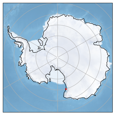
Extract and join together the latitude and longitude variables from the Platform group in the ed EchoData object. Convert to a Pandas DataFrame first, then to a GeoPandas GeoDataFrame for convenient viewing and manipulation.
# Create gps dataframe
gps_df = ed['Platform'].latitude.to_dataframe().join(ed['Platform'].longitude.to_dataframe())
gps_df.head(3)
| latitude | longitude | |
|---|---|---|
| time3 | ||
| 2018-01-11 07:26:30.393129984 | -75.018896 | 165.499855 |
| 2018-01-11 07:48:05.826169856 | -75.017433 | 165.500057 |
| 2018-01-11 07:48:06.832060160 | -75.017432 | 165.500058 |
# Create geodataframe from gps_df
gps_gdf = gpd.GeoDataFrame(
    gps_df,
    geometry=gpd.points_from_xy(gps_df['longitude'], gps_df['latitude']),
)

try:
    gps_gdf = gps_gdf.set_crs("EPSG:4326")
except Exception:
    gps_gdf = gps_gdf.set_crs("+proj=longlat +datum=WGS84 +no_defs +type=crs")
# Plot lat lon bounding box points
print("Minimum Longitude:", gps_df.longitude.min())
print("Maximum Longitude:", gps_df.longitude.max())
print("Minimum Latitude:", gps_df.latitude.min())
print("Maximum Latitude:", gps_df.latitude.max())
Minimum Longitude: 165.49765868921702
Maximum Longitude: 165.50005833333333
Minimum Latitude: -75.01889590423247
Maximum Latitude: -75.01737333333334
Using matplotlib and cartopy, plot the individual GPS points with a South Polar Stereo map projection.
# Plot on Polar Map
_, ax = plt.subplots(figsize=(5, 5), subplot_kw={"projection": ccrs.SouthPolarStereo()})
ax.set_extent([-180, 180, -90, -65], crs=ccrs.PlateCarree())
ax.coastlines(resolution='110m')
ax.stock_img()
ax.gridlines()
gps_gdf.plot(ax=ax, markersize=10, color='red', transform=ccrs.PlateCarree(), aspect=None)
<GeoAxes: >
Calibrate backscatter data with glider mean environmental data#
We’ll use the environmental data (temperature, salinity and pressure) found in the external glider file and the calibration parameters stored in the AZFP files to calibrate the backscatter data and create a volume backscattering strength (Sv) dataset.
# Grab and average environmental parameters
env_params_means = {}
for env_var in ["temperature", "salinity", "pressure"]:
    env_params_means[env_var] = float(ds_glider[env_var].mean().values)
env_params_means
{'temperature': -1.0206379890441895,
 'salinity': 34.53364181518555,
 'pressure': 38.69340133666992}
# Compute Sv
ds_Sv = ep.calibrate.compute_Sv(ed, env_params=env_params_means)
ds_Sv
<xarray.Dataset> Size: 88MB
Dimensions:                (channel: 3, ping_time: 920, range_sample: 1999,
                            filenames: 1)
Coordinates:
  * channel                (channel) <U11 132B '59006-38-1' ... '59006-200-3'
  * ping_time              (ping_time) datetime64[ns] 7kB 2018-01-11T07:44:40...
  * range_sample           (range_sample) int64 16kB 0 1 2 3 ... 1996 1997 1998
  * filenames              (filenames) int64 8B 0
Data variables: (12/18)
    Sv                     (channel, ping_time, range_sample) float64 44MB -1...
    echo_range             (channel, ping_time, range_sample) float64 44MB 0....
    frequency_nominal      (channel) float64 24B 3.8e+04 1.25e+05 2e+05
    sound_speed            float64 8B 1.444e+03
    sound_absorption       (channel) float64 24B 0.009111 0.03012 0.04501
    temperature            float64 8B -1.021
    ...                     ...
    TVR                    (channel) float64 24B 156.2 168.5 165.9
    VTX0                   (channel) float64 24B 157.0 146.7 133.3
    equivalent_beam_angle  (channel) float64 24B 0.1306 0.01071 0.01071
    Sv_offset              (channel) float64 24B 0.7 0.3 0.3
    source_filenames       (filenames) <U37 148B 'example_data/glider_AZFP/18...
    water_level            float64 8B nan
Attributes:
    processing_software_name:     echopype
    processing_software_version:  0.11.1
    processing_time:              2026-04-18T19:38:15+00:00
processing_function: calibrate.compute_Sv# Plot Sv
ds_Sv["Sv"].plot(
col="channel", yincrease=False, y="range_sample",
vmin=-100, vmax=-60, cmap="ep.ek500"
)
<xarray.plot.facetgrid.FacetGrid at 0x7f46dda750d0>
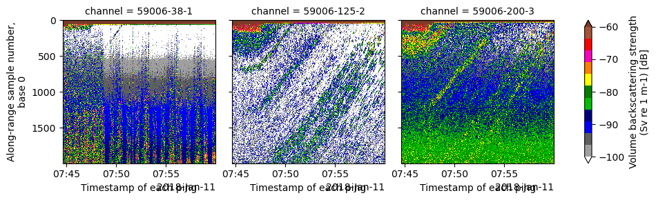
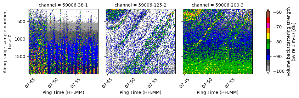
Note that the top portion of the echograms have extremely high Sv values. Let’s drop these since they are most likely from noise or bubbles near the sea surface.
# Select Sv
ds_Sv = ds_Sv.isel(range_sample=slice(150,None))
# Plot selected Sv:
g = ds_Sv["Sv"].plot(
    col="channel", yincrease=False, y="range_sample",
    vmin=-100, vmax=-60, cmap="ep.ek500"
)

# Iterate through each facet
for ax in g.axes.flatten():
    labels = [label.get_text() for label in ax.get_xticklabels()]
    # Set the current ticks
    ax.set_xticks(ax.get_xticks())
    # Apply rotation
    ax.set_xticklabels(labels, rotation=45)
    # Set x label
    ax.set_xlabel("Ping Time (HH:MM)")

plt.show()
/tmp/ipykernel_250/992655323.py:8: FutureWarning: self.axes is deprecated since 2022.11 in order to align with matplotlibs plt.subplots, use self.axs instead.
  for ax in g.axes.flatten():
Remove background noise#
Following De Robertis and Higginbottom (2007), we can remove background noise by estimating it from the mean calibrated power of a collection of pings.
# Remove background noise
ds_Sv = ep.clean.remove_background_noise(
    ds_Sv,
    ping_num=5,
    range_sample_num=5,
    # Threshold value from https://github.com/a-sheehan/Echopype-Processing-Pipeline-for-AZFP-and-Glider-Data/blob/main/Sheehan_azfp_forloop.ipynb
    SNR_threshold="2.0dB",
)
# Plot corrected Sv
g = ds_Sv["Sv_corrected"].plot(
    col="channel", yincrease=False, y="range_sample", vmin=-100, vmax=-60, cmap="ep.ek500"
)

# Iterate through each facet
for ax in g.axes.flatten():
    labels = [label.get_text() for label in ax.get_xticklabels()]
    # Set the current ticks
    ax.set_xticks(ax.get_xticks())
    # Apply rotation
    ax.set_xticklabels(labels, rotation=45)
    # Set x label
    ax.set_xlabel("Ping Time (HH:MM)")

plt.show()
/tmp/ipykernel_250/3887182110.py:7: FutureWarning: self.axes is deprecated since 2022.11 in order to align with matplotlibs plt.subplots, use self.axs instead.
  for ax in g.axes.flatten():
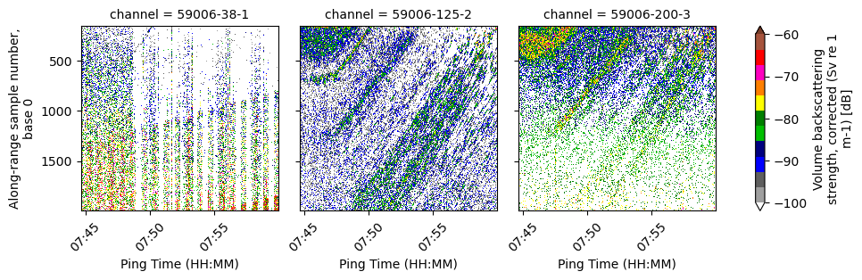
Since we’re most interested in 125 kHz for capturing zooplankton schools, let’s look at the Sv histograms (with and without background noise removed) for the 125 kHz channels:
# Extract and flatten data from 125 kHz channels
data_Sv = ds_Sv["Sv"].sel(channel="59006-125-2").values.ravel() # Flatten
data_Sv_corrected = ds_Sv["Sv_corrected"].sel(channel="59006-125-2").values.ravel() # Flatten

# Create a figure and axis
fig, ax = plt.subplots(figsize=(8, 5))

# Plot histograms
ax.hist(data_Sv, bins=100, color='blue', alpha=0.2, label='125 kHz Sv')
ax.hist(data_Sv_corrected, bins=100, color='red', alpha=0.2, label='Corrected 125 kHz Sv')

# Add labels, title, and legend
ax.set_xlabel("Volume backscattering strength (Sv re 1 m-1)[dB]")
ax.set_ylabel("Sv Value Frequency")
ax.set_title("Histogram Comparison between original Sv and background noise removed Sv")
ax.legend()

plt.show()
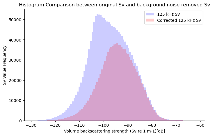
From both the histogram and the echogram images above, we can see that a significant amount of Sv values, between -120 and -90 dB, surrounding the orange and yellow regions in the 125 kHz channel have been removed. Being that the majority of values removed were so weak, we suspect that it was mostly background noise that was removed.
Align echosounder data according to depth#
What are range_sample and echo_range?#
Since the glider is going downwards, displaying the echogram as we did in the Sv plots above is not correct since it does not display the backscatter at its respective depth. For Sv, we have range_sample which is the number of samples a particular echo samples measured starting from the moment the ping was transmitted.
# Show `range_sample`
ds_Sv["range_sample"]
<xarray.DataArray 'range_sample' (range_sample: 1849)> Size: 15kB
array([ 150,  151,  152, ..., 1996, 1997, 1998], shape=(1849,))
Coordinates:
  * range_sample  (range_sample) int64 15kB 150 151 152 153 ... 1996 1997 1998
Attributes:
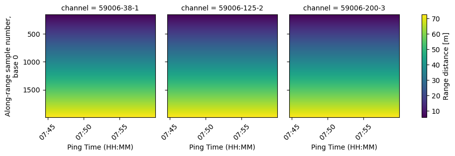
long_name: Along-range sample number, base 0To get the actual range (distance) of how far this echo pixel is from the transducer surface, the Sv dataset object also contains the echo_range variable that is calculated based on the sound speed (calculated from the environmental data) and sampling interval:
# Show `echo_range`
ds_Sv["echo_range"]
<xarray.DataArray 'echo_range' (channel: 3, ping_time: 920, range_sample: 1849)> Size: 41MB
array([[[ 5.77733777,  5.81344613,  5.84955449, ..., 72.43337229,
         72.46948066, 72.50558902],
        [ 5.77733777,  5.81344613,  5.84955449, ..., 72.43337229,
         72.46948066, 72.50558902],
        [ 5.77733777,  5.81344613,  5.84955449, ..., 72.43337229,
         72.46948066, 72.50558902],
        ...,
        [ 5.77733777,  5.81344613,  5.84955449, ..., 72.43337229,
         72.46948066, 72.50558902],
        [ 5.77733777,  5.81344613,  5.84955449, ..., 72.43337229,
         72.46948066, 72.50558902],
        [ 5.77733777,  5.81344613,  5.84955449, ..., 72.43337229,
         72.46948066, 72.50558902]],

       [[ 5.77733777,  5.81344613,  5.84955449, ..., 72.43337229,
         72.46948066, 72.50558902],
        [ 5.77733777,  5.81344613,  5.84955449, ..., 72.43337229,
         72.46948066, 72.50558902],
        [ 5.77733777,  5.81344613,  5.84955449, ..., 72.43337229,
         72.46948066, 72.50558902],
...
        [ 5.77733777,  5.81344613,  5.84955449, ..., 72.43337229,
         72.46948066, 72.50558902],
        [ 5.77733777,  5.81344613,  5.84955449, ..., 72.43337229,
         72.46948066, 72.50558902],
        [ 5.77733777,  5.81344613,  5.84955449, ..., 72.43337229,
         72.46948066, 72.50558902]],

       [[ 5.77733777,  5.81344613,  5.84955449, ..., 72.43337229,
         72.46948066, 72.50558902],
        [ 5.77733777,  5.81344613,  5.84955449, ..., 72.43337229,
         72.46948066, 72.50558902],
        [ 5.77733777,  5.81344613,  5.84955449, ..., 72.43337229,
         72.46948066, 72.50558902],
        ...,
        [ 5.77733777,  5.81344613,  5.84955449, ..., 72.43337229,
         72.46948066, 72.50558902],
        [ 5.77733777,  5.81344613,  5.84955449, ..., 72.43337229,
         72.46948066, 72.50558902],
        [ 5.77733777,  5.81344613,  5.84955449, ..., 72.43337229,
         72.46948066, 72.50558902]]], shape=(3, 920, 1849))
Coordinates:
  * channel       (channel) <U11 132B '59006-38-1' '59006-125-2' '59006-200-3'
  * ping_time     (ping_time) datetime64[ns] 7kB 2018-01-11T07:44:40 ... 2018...
  * range_sample  (range_sample) int64 15kB 150 151 152 153 ... 1996 1997 1998
Attributes:
    long_name:  Range distance
units: m# Plot `echo_range`
g = ds_Sv["echo_range"].plot(col="channel", y="range_sample", yincrease=False)
# Iterate through each facet
for ax in g.axes.flatten():
labels = [label.get_text() for label in ax.get_xticklabels()]
# Set the current ticks
ax.set_xticks(ax.get_xticks())
# Apply rotation
ax.set_xticklabels(labels, rotation=45)
# Set x label
ax.set_xlabel("Ping Time (HH:MM)")
plt.show()
/tmp/ipykernel_250/3346364644.py:5: FutureWarning: self.axes is deprecated since 2022.11 in order to align with matplotlibs plt.subplots, use self.axs instead.
  for ax in g.axes.flatten():
# Show `echo_range` dimensions
ds_Sv["echo_range"].dims
('channel', 'ping_time', 'range_sample')
This is a 3D array, with the same dimensions as the Sv array. In this case, the echo_range is equal across channels and pings; however, this is not always the case and so we have to construct the echo_range variable as a 3D array.
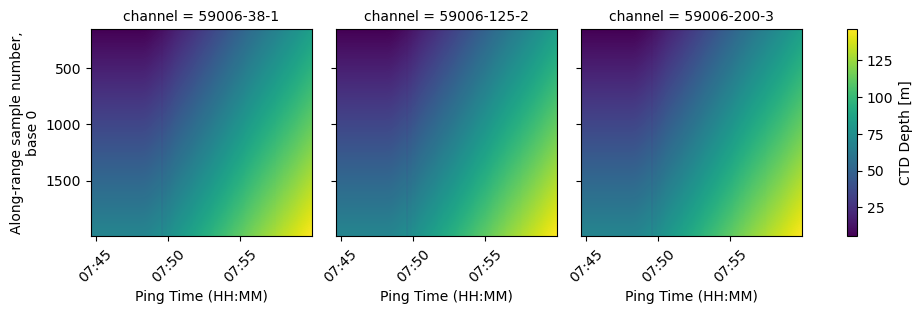
Since echo_range is calculated from the surface of the transducer, we can use the echo_range variable and external parameters to compute a depth array that captures this downward movement of the glider and position the echogram at the right depth.
Adding depth to Sv#
We can use external parameters from the ds_glider to compute depth.
We must first convert the glider dataset’s pitch and roll, which are in radians, into tilt, which is in degrees.
# Correct pitch based on the processing from:
# https://github.com/a-sheehan/Echopype-Processing-Pipeline-for-AZFP-and-Glider-Data/blob/main/Sheehan_azfp_forloop.ipynb
correct_pitch = ds_glider["m_pitch"].where(
    (ds_glider["m_pitch"]*180/np.pi < -15) & (ds_glider["m_pitch"]*180/np.pi > -30),
    other=np.nan
)

# Convert pitch and roll from radians to degrees
pitch = np.rad2deg(correct_pitch)
roll = np.rad2deg(ds_glider["m_roll"])

# Compute tilt in degrees from pitch roll rotations
yaw = np.zeros_like(pitch.values)
yaw_pitch_roll_euler_angles_stack = np.column_stack([yaw, pitch.values, roll.values])
yaw_rot_pitch_roll = R.from_euler("ZYX", yaw_pitch_roll_euler_angles_stack, degrees=True)
glider_tilt = yaw_rot_pitch_roll.as_matrix()[:, -1, -1]
glider_tilt = xr.DataArray(
    glider_tilt, dims="time", coords={"time": ds_glider["time"]}
)
glider_tilt_in_degrees = np.rad2deg(np.arccos(glider_tilt))
glider_tilt_in_degrees.attrs = {
    "long_name": "Tilt",
    "units": "Degrees"
}
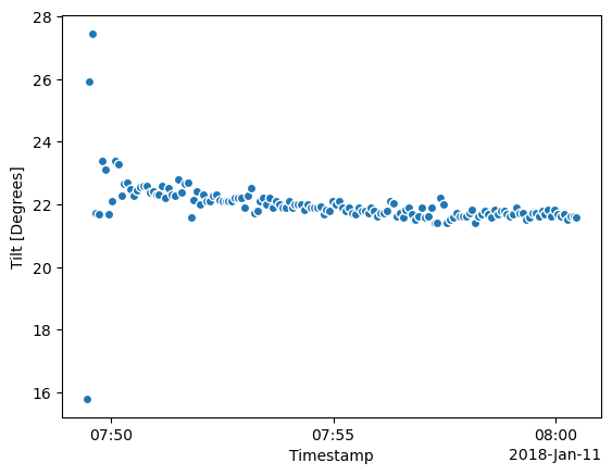
Plotting glider tilt:
# Plot glider tilt
glider_tilt_in_degrees.plot.scatter()
<matplotlib.collections.PathCollection at 0x7f46e4c2f090>
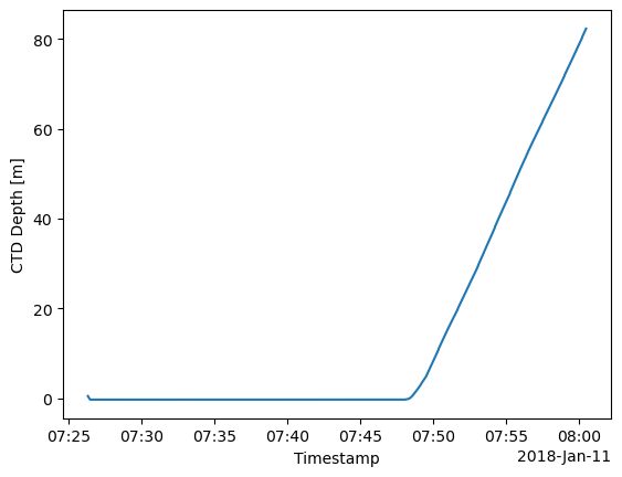
Plotting glider specified depth:
# Plot glider depth
ds_glider["depth"].dropna(dim="time").plot.line()
[<matplotlib.lines.Line2D at 0x7f46e0bc3090>]
We use both angular and vertical offset information alongside echo_range in ep.consolidate.add_depth to correctly compute the depth that each backscatter data point corresponds to:
# Add depth to Sv dataset incorporating Glider depth and tilt data
ds_Sv = ep.consolidate.add_depth(
    ds_Sv,
    depth_offset=ds_glider["depth"].dropna("time"),
    tilt=glider_tilt_in_degrees.dropna("time"),
)
Plot the depth array:
# Plot the depth array
g = ds_Sv["depth"].plot(col="channel", y="range_sample", yincrease=False)

# Iterate through each facet
for ax in g.axes.flatten():
    labels = [label.get_text() for label in ax.get_xticklabels()]
    # Set the current ticks
    ax.set_xticks(ax.get_xticks())
    # Apply rotation
    ax.set_xticklabels(labels, rotation=45)
    # Set x label
    ax.set_xlabel("Ping Time (HH:MM)")

plt.show()
/tmp/ipykernel_250/2361482427.py:5: FutureWarning: self.axes is deprecated since 2022.11 in order to align with matplotlibs plt.subplots, use self.axs instead.
  for ax in g.axes.flatten():
Plot the 125 kHz channel of the Sv corrected dataset using depth as a 2D coordinate grid:
# Create a single subplot
fig, ax = plt.subplots(1,1,figsize=(12,6))

# Plot 125 kHz Sv corrected channel as a 2D mesh with depth and ping time coords
pcolormesh = plt.pcolormesh(
    ds_Sv["ping_time"].broadcast_like(ds_Sv["range_sample"]).values.T,
    ds_Sv["depth"].sel(channel="59006-125-2").values,
    ds_Sv["Sv_corrected"].sel(channel="59006-125-2").values,
    shading='auto',
    vmin=-100,
    vmax=-60,
    cmap="ep.ek500",
)
plt.gca().invert_yaxis()

# Add title and axis labels
plt.title("125 kHz Sv (with background noise removed)")
plt.xlabel("Ping Time (DD HH:MM)")
plt.ylabel("Depth (m)")

# Add colorbar
plt.colorbar(pcolormesh, label="Volume backscattering strength (Sv re 1 m-1)[dB]")

# Show plot
plt.show()
/tmp/ipykernel_250/3509394515.py:5: UserWarning: The input coordinates to pcolormesh are interpreted as cell centers, but are not monotonically increasing or decreasing. This may lead to incorrectly calculated cell edges, in which case, please supply explicit cell edges to pcolormesh.
  pcolormesh = plt.pcolormesh(
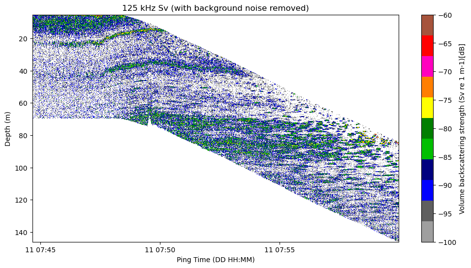
Note that the first few roll and pitch angles may be inaccurate, and hence there is a small “jump” near the start of the dive in the depth of the echogram.
Compute and apply shoal mask on corrected Sv#
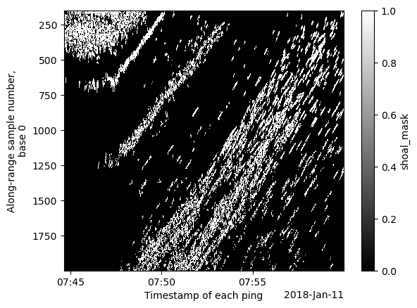
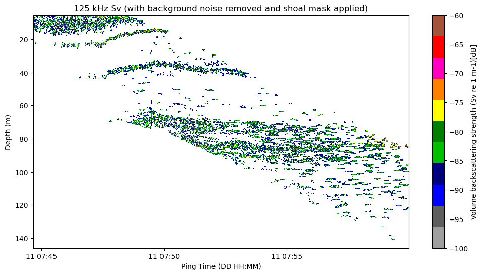
With the calibrated backscatter volume data in an easily manipulable array format, here we use echopype’s shoal detection functionality to extract the zooplankton schools seen in the echogram above. There are multiple options to perform shoal detection, and below we use the one used by Echoview, with the implementation adapted from another open-source fisheries acoustics package, Echopy.
from echopype.mask import detect_shoal

shoal_mask = detect_shoal(
    ds_Sv,
    method="echoview",
    params={
        "var_name": "Sv_corrected",
        "channel": "59006-125-2",
        "idim": np.arange(len(ds_Sv["range_sample"])+1),
        "jdim": np.arange(len(ds_Sv["ping_time"])+1),
        "thr": -90,
        "mincan": (5, 5),
        "maxlink": (30, 2),
        "minsho": (30, 2),
    }
)
The mask is binary, where 1 is within a zooplankton school, and 0 otherwise:
# Plot the school mask
shoal_mask.plot(yincrease=False, y="range_sample", cmap="gray")
<matplotlib.collections.QuadMesh at 0x7f46e6d69010>
# Apply shoal mask on the corrected Sv
ds_shoal_masked_Sv = ep.mask.apply_mask(ds_Sv, shoal_mask, var_name="Sv_corrected")
Plot the 125 kHz channel of the shoal masked Sv dataset using depth as a 2D coordinate grid:
# Create a single subplot
fig, ax = plt.subplots(1,1,figsize=(12,6))

# Plot shoal masked 38 kHz Sv channel as a 2D mesh with depth and ping time coords
pcolormesh = plt.pcolormesh(
    ds_shoal_masked_Sv["ping_time"].broadcast_like(ds_shoal_masked_Sv["range_sample"]).values.T,
    ds_shoal_masked_Sv["depth"].sel(channel="59006-125-2").values,
    ds_shoal_masked_Sv["Sv_corrected"].sel(channel="59006-125-2").values,
    shading='auto',
    vmin=-100,
    vmax=-60,
    cmap="ep.ek500",
)
plt.gca().invert_yaxis()

# Add title and axis labels
plt.title("125 kHz Sv (with background noise removed and shoal mask applied)")
plt.xlabel("Ping Time (DD HH:MM)")
plt.ylabel("Depth (m)")

# Add colorbar
plt.colorbar(pcolormesh, label="Volume backscattering strength (Sv re 1 m-1)[dB]")

# Show plot
plt.show()
/tmp/ipykernel_250/2654804491.py:5: UserWarning: The input coordinates to pcolormesh are interpreted as cell centers, but are not monotonically increasing or decreasing. This may lead to incorrectly calculated cell edges, in which case, please supply explicit cell edges to pcolormesh.
  pcolormesh = plt.pcolormesh(
Package versions#
import datetime
print(f"echopype: {ep.__version__}, xarray: {xr.__version__}, geopandas: {gpd.__version__}")

print(f"\n{datetime.datetime.utcnow()} +00:00")
echopype: 0.11.1, xarray: 2026.2.0, geopandas: 1.1.2

2026-04-18 19:42:11.009823 +00:00