Incorporate an external mask to compute NASC attributed to Pacific hake from ship echosounder data

This notebook accompanies the following paper:

Echopype: Interoperable and scalable echosounder data processing with Echopype
Authors: Wu-Jung Lee, Landung Setiawan, Caesar Tuguinay, Emilio Mayorga, and Valentina Staneva
ICES Journal of Marine Science 2024: https://doi.org/10.1093/icesjms/fsae133

Introduction

Description

This notebook uses a small subset of the EK60 echosounder data collected during the 2017 Joint U.S.-Canada Integrated Ecosystem and Pacific Hake Acoustic Trawl Survey (aka the “Hake survey”) to illustrate a processing pipeline that compute Nautical Areal Scattering Coefficient (NASC) attributed to Pacific hake. The workflow includes steps to perform data conversion, calibration, regridding, and masking, using functions from Echopype, and core scientific Python software packages, particularly NumPy, Xarray, and Dask. This workflow utilizes hake annotations which were manually produced from the NOAA Fisheries Northwest Fisheries Science Center (NWFSC) Fisheries Engineering and Acoustic Technologies Team (FEAT).

Outline

1. Convert EK60 .raw files to EchoData Objects

2. Combine EchoData Objects

3. Calibrate raw backscatter measurement in the combined EchoData object to Sv

4. Read and apply a binary mask for Pacific hake presence

5. Compute and plot NASC attributed to Pacific hake

Running the notebook

This notebook can be run with a conda environment created using the conda environment file. The notebook creates a directory, if not already present: ./exports/hake_mask. All Zarr files will be exported there.

Note

We encourage importing Echopype as ep for consistency.

from pathlib import Path
import os

import xarray as xr
import numpy as np
import matplotlib.pyplot as plt

from dask.distributed import Client

import echopype as ep
from echopype import colormap # needed for the EK500 colormap

import warnings
warnings.simplefilter("ignore", category=DeprecationWarning)
# Ignore large graph dask UserWarnings
warnings.simplefilter("ignore", category=UserWarning)

Setup

Path setup

Set paths and create directories to store Zarr files:

import_path = Path("example_data/NWFSC_2017_hake_survey_transect_with_hake/")

output_path = Path("./exports/hake_mask")
output_path.mkdir(exist_ok=True, parents=True)

echodata_zarr_path = output_path / "echodata_zarr"
echodata_zarr_path.mkdir(exist_ok=True)
combined_zarr_path = output_path / "combined_zarr"
combined_zarr_path.mkdir(exist_ok=True)

Dask Client setup

Echopype leverages Dask’s lazy-load mechanisms to perform out-of-core and parallelized computation on large datasets. We use the Dask Client that is pointed to a Scheduler that schedules tasks and allocate memory for these computations.

# Use maximum number of CPUs for Dask Client
client = Client() # Set n_workers so that total_RAM / n_workers >= 4
                  # or leave empty and let Dask decide
print("Dask Client Dashboard:", client.dashboard_link)

Dask Client Dashboard: http://127.0.0.1:8787/status

Click on the Dask Client Dashboard link above to view the computations live.

For more information on how to use, view, and interpret the Dashboard, go to this link: https://docs.dask.org/en/stable/dashboard.html

Data processing workflow

The following data processing steps follow the typical Echopype workflow, which converts and standardizes data before performing more computation. Below we first convert and save the .raw files generated by EK60 to Zarr stores on disk, and lazy-load them back for downstream processing. This allows us to perform computations that may require resources that are larger than the local system memory.

Identify target echosounder data files

Identify EK60 .raw files associated with the first segment of transect 45 of the 2017 survey:

ncei_2017_ek60_raws_path = "ncei-wcsd-archive/data/raw/Bell_M._Shimada/SH1707/EK60"
transect_name = "x0045_0_wt_20170717_213507_f0010"
transect_file_paths = []
with open(import_path / transect_name, 'r') as file:
    for line in file:
        transect_file_paths.append(
            f"{ncei_2017_ek60_raws_path}/{line.strip()}.raw"
        )

transect_file_paths

['ncei-wcsd-archive/data/raw/Bell_M._Shimada/SH1707/EK60/Summer2017-D20170717-T212115.raw',
 'ncei-wcsd-archive/data/raw/Bell_M._Shimada/SH1707/EK60/Summer2017-D20170717-T214833.raw',
 'ncei-wcsd-archive/data/raw/Bell_M._Shimada/SH1707/EK60/Summer2017-D20170717-T221909.raw',
 'ncei-wcsd-archive/data/raw/Bell_M._Shimada/SH1707/EK60/Summer2017-D20170717-T224632.raw',
 'ncei-wcsd-archive/data/raw/Bell_M._Shimada/SH1707/EK60/Summer2017-D20170717-T231028.raw',
 'ncei-wcsd-archive/data/raw/Bell_M._Shimada/SH1707/EK60/Summer2017-D20170717-T233247.raw',
 'ncei-wcsd-archive/data/raw/Bell_M._Shimada/SH1707/EK60/Summer2017-D20170717-T235306.raw',
 'ncei-wcsd-archive/data/raw/Bell_M._Shimada/SH1707/EK60/Summer2017-D20170718-T001206.raw',
 'ncei-wcsd-archive/data/raw/Bell_M._Shimada/SH1707/EK60/Summer2017-D20170718-T003054.raw',
 'ncei-wcsd-archive/data/raw/Bell_M._Shimada/SH1707/EK60/Summer2017-D20170718-T004846.raw']

These RAW files combined are about ~250 MB in size.

Convert EK60 .raw files to EchoData objects

%%time

# Save Echodata objects locally
def open_and_save(raw_file, sonar_model, use_swap, save_path, storage_options):
    try:
        ed = ep.open_raw(
            raw_file=f's3://{raw_file}',
            sonar_model=sonar_model,
            use_swap=use_swap,
            storage_options=storage_options,
        )
        ed.to_zarr(save_path, overwrite=True, compute=True)
    except Exception as e:
        print("Error with Exception: ", e)

# Parse EK60 `.RAW` file and save to Zarr Store
open_and_save_futures = []
for raw_file_url in transect_file_paths:
    open_and_save_future = client.submit(
        open_and_save,
        raw_file=raw_file_url,
        sonar_model='ek60',
        use_swap=True,
        save_path=echodata_zarr_path,
        storage_options={'anon': True}
    )
    open_and_save_futures.append(open_and_save_future)
open_and_save_futures = client.gather(open_and_save_futures)

CPU times: user 796 ms, sys: 93.2 ms, total: 889 ms
Wall time: 9.4 s

Combine EchoData objects

Under the hood of the ep.combine_echodata function, the Zarr stores of each EchoData object are loaded and appended lazily, meaning that no data loading or appending actually happens until the combined object is saved to disk via to_zarr. Since the EchoData is appended sequentially based on the data time sequence and therefore not parallelized, this is the slowest stage of the processing pipeline.

%%time

# Open (lazy-load) Zarr stores containing EchoData Objects, and lazily combine them
ed_future_list = []
for converted_file in sorted(echodata_zarr_path.glob("*.zarr")):
    ed_future = client.submit(    
        ep.open_converted,
        converted_raw_path=converted_file,
        chunks={}
    )
    ed_future_list.append(ed_future)
ed_list = client.gather(ed_future_list)
ed_combined = ep.combine_echodata(ed_list)

# Save the combined EchoData object to a new Zarr store
# The appending operation only happens when relevant data needs to be save to disk
ed_combined.to_zarr(
    combined_zarr_path / "ed_combined.zarr",
    overwrite=True,
    compute=True,
)

# Lazy-load the comined Zarr store
ed_combined = ep.open_converted(
    combined_zarr_path / "ed_combined.zarr",
    chunks={},
)

CPU times: user 7.99 s, sys: 633 ms, total: 8.62 s
Wall time: 13.8 s

Calibrate raw backscatter measurement in the combined EchoData object to Sv

Compute Volume Backscattering Strength (Sv) from raw backscatter measurements stored in the converted EchoData object, and add depth and latitude/longitude to this Xarray Dataset.

%%time

# Chunk EchoData object ping-wise
ed_combined = ed_combined.chunk({"ping_time": 1000, "range_sample": -1})

# Compute Sv
ds_Sv = ep.calibrate.compute_Sv(ed_combined)

# Add Depth
ds_Sv = ep.consolidate.add_depth(ds_Sv, depth_offset=9.15)

# Add Latitude and Longitude
ds_Sv = ep.consolidate.add_location(ds_Sv, ed_combined)

# Save to Zarr and offload computation to disk
ds_Sv.to_zarr(
    combined_zarr_path / "ds_Sv.zarr",
    mode="w",
    compute=True,
)

# Lazy-load the Zarr store
ds_Sv = xr.open_dataset(
    combined_zarr_path / "ds_Sv.zarr",
    engine="zarr",
    chunks={},
)

CPU times: user 1.45 s, sys: 101 ms, total: 1.55 s
Wall time: 3.27 s

print("Sv dimensions:", ds_Sv["Sv"].dims)

Sv dimensions: ('channel', 'ping_time', 'range_sample')

print("Depth dimensions:", ds_Sv["depth"].dims)

Depth dimensions: ('channel', 'ping_time', 'range_sample')

g = ds_Sv["depth"].plot(col="channel", y="range_sample", yincrease=False)

# Iterate through each facet
for ax in g.axes.flatten():
    labels = [label.get_text() for label in ax.get_xticklabels()]
    # Set the current ticks
    ax.set_xticks(ax.get_xticks())
    # Apply rotation
    ax.set_xticklabels(labels, rotation=45)
    # Set x label
    ax.set_xlabel("Ping Time (HH:MM)")

plt.show()

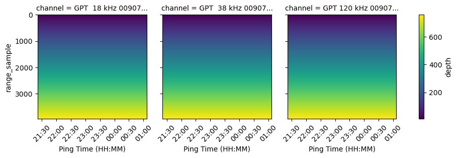
In general, hand drawn annotations for hake contain depth information that isn’t aligned with the range_sample dimension of the volume backscatter dataset.

To accomodate for this, we have to swap the range_sample dimension with the depth dimension. Generally, this is not allowed since the depth variable is a 3D variable (with dimensions channel, range_sample, and ping_time) and the range_sample variable is a 1D variable. However, as can be seen above, depth is equal across channel and ping time. This being the case, we can choose the depth vector corresponding to the first ping time and the first channel and set that as our new depth dimension:

# Create Sv dataset with depth dimension:
ds_Sv_with_depth_dim = ds_Sv.copy()
depth_1d = ds_Sv_with_depth_dim["depth"].isel(channel=0, ping_time=0)
ds_Sv_with_depth_dim["depth"] = depth_1d
ds_Sv_with_depth_dim = ds_Sv_with_depth_dim.swap_dims({"range_sample": "depth"})

Regrid calibrated data

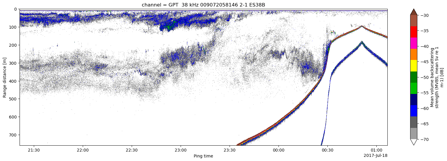
Compute mean volume backscattering strength (MVBS), which are binned averages of Sv (in the linear domain) across ping time and depth. This gets the data onto a common grid from the original ping time and depth sample size that may vary across ping and channel depending on the echosounder setting.

%%time

# Compute MVBS
ds_MVBS = ep.commongrid.compute_MVBS(
    ds_Sv,
    range_var="depth",
    range_bin='1m',  # in meters
    ping_time_bin='5s',  # in seconds
)

# Save to Zarr and offload computation to disk
ds_MVBS.to_zarr(
    combined_zarr_path / "ds_MVBS.zarr",
    mode="w",
    compute=True,
)

# Lazy-load the Zarr store
ds_MVBS = xr.open_dataset(
    combined_zarr_path / "ds_MVBS.zarr",
    engine="zarr",
    chunks={},
)

CPU times: user 2.08 s, sys: 114 ms, total: 2.2 s
Wall time: 11.2 s

plt.figure(figsize = (20, 6))
# Plot MVBS from the 38kHz channel
ds_MVBS["Sv"].sel(
    channel="GPT  38 kHz 009072058146 2-1 ES38B"
).plot.pcolormesh(
    y="depth",
    yincrease=False,
    vmin=-70,
    vmax=-30,
    cmap="ep.ek500",
)

<matplotlib.collections.QuadMesh at 0x700ad1414100>

Read and apply a binary mask for Pacific hake presence

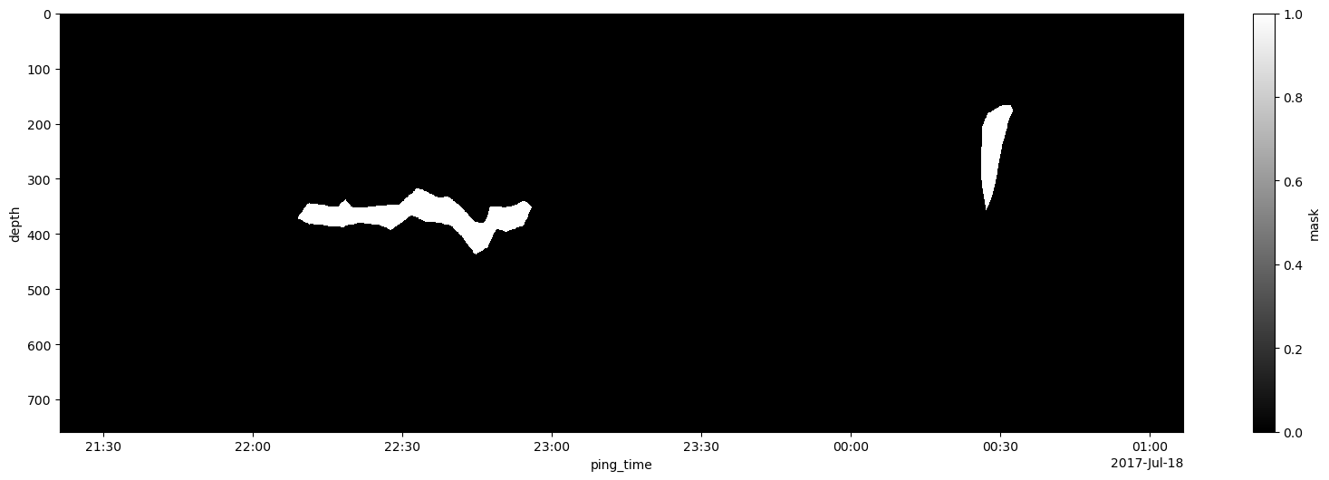
The mask was created based on annotations by the NOAA NWFSC FEAT team, and processed with the Echoregions package and stored as a boolean array. There were several steps needed to produce this mask from region annotations: excluding echogram pixels containing seafloor echoes, ensuring the regions are within transect, and regridding. For more details readers can refer to the Echoregions documentation.

hake_mask = xr.open_dataarray(
    "example_data/NWFSC_2017_hake_survey_transect_with_hake/hake_mask.nc",
    engine="netcdf4",
)

plt.figure(figsize = (20, 6))
hake_mask.plot(x='ping_time', y="depth", cmap='gray', yincrease=False)

<matplotlib.collections.QuadMesh at 0x700ad1327340>

# Check that MVBS and regridded clean hake mask match on depth and ping time dimensions:
assert hake_mask["depth"].equals(ds_MVBS["depth"])
assert hake_mask["ping_time"].equals(ds_MVBS["ping_time"])

In this case the coordinates of the mask and MVBS are matching. If not, one would need to align the mask with the ep.commongrid functions.

# Apply the mask to ds_MVBS
ds_MVBS_hake = ep.mask.apply_mask(ds_MVBS, hake_mask)

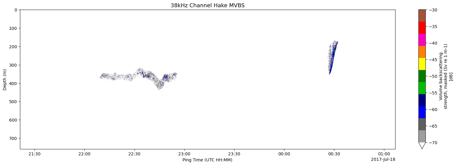
Let’s check the 38 kHz channel of the masked MVBS dataset:

# Add attributes to depth and ping time
ds_MVBS_hake["depth"].attrs["long_name"] = "Depth (m)"
ds_MVBS_hake["ping_time"].attrs["long_name"] = "Ping Time (UTC HH:MM)"

# Plot 38 kHz MVBS attributed to Clean Hake
p = ds_MVBS_hake["Sv"].sel(
    channel='GPT  38 kHz 009072058146 2-1 ES38B'
).plot.pcolormesh(
    y="depth",
    yincrease=False,
    vmin=-70,
    vmax=-30,
    cmap="ep.ek500",
    figsize=(20, 6)
)

# Set axes title
p.axes.set_title("38kHz Channel Hake MVBS", fontsize=13)

# Show plot
plt.show()

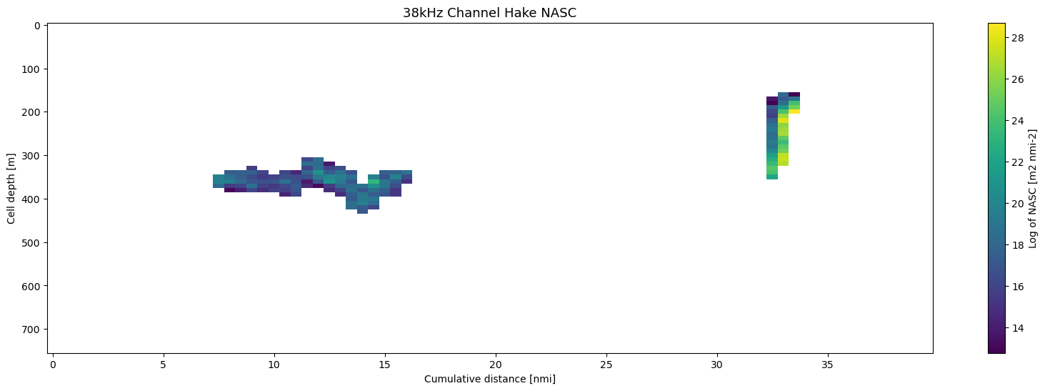
Compute and plot NASC attributed to Pacific hake

# Compute NASC from the masked MVBS dataset
ds_NASC = ep.commongrid.compute_NASC(
    ds_MVBS_hake,
    range_bin="10m",
    dist_bin="0.5nmi"
)

# Log-transform the NASC values for plotting
ds_NASC["NASC_log"] = 10 * np.log10(ds_NASC["NASC"])
ds_NASC["NASC_log"].attrs = {
    "long_name": "Log of NASC",
    "units": "m2 nmi-2"
}

# Show the hake NASC dataset
ds_NASC

<xarray.Dataset> Size: 295kB
Dimensions:            (channel: 3, distance: 80, depth: 76)
Coordinates:
  * distance           (distance) float64 640B 0.0 0.5 1.0 ... 38.5 39.0 39.5
  * channel            (channel) <U37 444B 'GPT  18 kHz 009072058c8d 1-1 ES18...
  * depth              (depth) float64 608B 0.0 10.0 20.0 ... 730.0 740.0 750.0
Data variables:
    NASC               (channel, distance, depth) float64 146kB dask.array<chunksize=(3, 80, 76), meta=np.ndarray>
    latitude           (distance) float64 640B dask.array<chunksize=(80,), meta=np.ndarray>
    longitude          (distance) float64 640B dask.array<chunksize=(80,), meta=np.ndarray>
    ping_time          (distance) datetime64[ns] 640B 2017-07-17T21:23:22.500...
    frequency_nominal  (channel) float64 24B dask.array<chunksize=(3,), meta=np.ndarray>
    NASC_log           (channel, distance, depth) float64 146kB dask.array<chunksize=(3, 80, 76), meta=np.ndarray>
Attributes:
    Conventions:           CF-1.7,ACDD-1.3
    time_coverage_start:   2017-07-17T21:21:15.000000000Z
    time_coverage_end:     2017-07-18T01:06:35.000000000Z
    geospatial_lat_min:    41.79633
    geospatial_lat_max:    41.82402
    geospatial_lon_min:    -125.21041
    geospatial_lon_max:    -124.41516
    processing_level:      Level 4
    processing_level_url:  https://echopype.readthedocs.io/en/stable/processi...

xarray.Dataset

• Dimensions:
  • channel: 3
  • distance: 80
  • depth: 76
• Coordinates: (3)
  • distance
    (distance)
    float64
    0.0 0.5 1.0 1.5 ... 38.5 39.0 39.5

    long_name :

    Cumulative distance

    units :

    nmi

    actual_range :

    [0.0, 39.5]

    array([ 0. ,  0.5,  1. ,  1.5,  2. ,  2.5,  3. ,  3.5,  4. ,  4.5,  5. ,  5.5,
            6. ,  6.5,  7. ,  7.5,  8. ,  8.5,  9. ,  9.5, 10. , 10.5, 11. , 11.5,
           12. , 12.5, 13. , 13.5, 14. , 14.5, 15. , 15.5, 16. , 16.5, 17. , 17.5,
           18. , 18.5, 19. , 19.5, 20. , 20.5, 21. , 21.5, 22. , 22.5, 23. , 23.5,
           24. , 24.5, 25. , 25.5, 26. , 26.5, 27. , 27.5, 28. , 28.5, 29. , 29.5,
           30. , 30.5, 31. , 31.5, 32. , 32.5, 33. , 33.5, 34. , 34.5, 35. , 35.5,
           36. , 36.5, 37. , 37.5, 38. , 38.5, 39. , 39.5])

  • channel
    (channel)
    <U37
    'GPT 18 kHz 009072058c8d 1-1 ES...

    array(['GPT  18 kHz 009072058c8d 1-1 ES18-11',
           'GPT  38 kHz 009072058146 2-1 ES38B',
           'GPT 120 kHz 00907205a6d0 4-1 ES120-7C'], dtype='<U37')

  • depth
    (depth)
    float64
    0.0 10.0 20.0 ... 730.0 740.0 750.0

    long_name :

    Cell depth

    units :

    m

    actual_range :

    [0.0, 750.0]

    standard_name :

    depth

    array([  0.,  10.,  20.,  30.,  40.,  50.,  60.,  70.,  80.,  90., 100., 110.,
           120., 130., 140., 150., 160., 170., 180., 190., 200., 210., 220., 230.,
           240., 250., 260., 270., 280., 290., 300., 310., 320., 330., 340., 350.,
           360., 370., 380., 390., 400., 410., 420., 430., 440., 450., 460., 470.,
           480., 490., 500., 510., 520., 530., 540., 550., 560., 570., 580., 590.,
           600., 610., 620., 630., 640., 650., 660., 670., 680., 690., 700., 710.,
           720., 730., 740., 750.])

• Data variables: (6)
  • NASC
    (channel, distance, depth)
    float64
    dask.array<chunksize=(3, 80, 76), meta=np.ndarray>

    long_name :

    Nautical Areal Scattering Coefficient (NASC, m2 nmi-2)

    units :

    m2 nmi-2

    actual_range :

    [6.24, 1888.884]

    Array Chunk Bytes 142.50 kiB 142.50 kiB Shape (3, 80, 76) (3, 80, 76) Dask graph 1 chunks in 18 graph layers Data type float64 numpy.ndarray

  • latitude
    (distance)
    float64
    dask.array<chunksize=(80,), meta=np.ndarray>

    history :

    2024-08-08 23:14:23.948010 +00:00. Interpolated or propagated from Platform latitude/longitude.

    long_name :

    Platform latitude

    standard_name :

    latitude

    units :

    degrees_north

    valid_range :

    (-90.0, 90.0)

    Array Chunk Bytes 640 B 640 B Shape (80,) (80,) Dask graph 1 chunks in 6 graph layers Data type float64 numpy.ndarray

  • longitude
    (distance)
    float64
    dask.array<chunksize=(80,), meta=np.ndarray>

    history :

    2024-08-08 23:14:23.948010 +00:00. Interpolated or propagated from Platform latitude/longitude.

    long_name :

    Platform longitude

    standard_name :

    longitude

    units :

    degrees_east

    valid_range :

    (-180.0, 180.0)

    Array Chunk Bytes 640 B 640 B Shape (80,) (80,) Dask graph 1 chunks in 6 graph layers Data type float64 numpy.ndarray

  • ping_time
    (distance)
    datetime64[ns]
    2017-07-17T21:23:22.500000 ... 2...

    long_name :

    Ping Time (UTC HH:MM)

    array(['2017-07-17T21:23:22.500000000', '2017-07-17T21:27:47.500000000',
           '2017-07-17T21:32:10.000000000', '2017-07-17T21:36:00.000000000',
           '2017-07-17T21:39:05.000000000', '2017-07-17T21:41:50.000000000',
           '2017-07-17T21:44:30.000000000', '2017-07-17T21:47:10.000000000',
           '2017-07-17T21:49:52.500000000', '2017-07-17T21:52:32.500000000',
           '2017-07-17T21:55:12.500000000', '2017-07-17T21:57:57.500000000',
           '2017-07-17T22:00:45.000000000', '2017-07-17T22:03:32.500000000',
           '2017-07-17T22:06:20.000000000', '2017-07-17T22:09:05.000000000',
           '2017-07-17T22:11:52.500000000', '2017-07-17T22:14:40.000000000',
           '2017-07-17T22:17:25.000000000', '2017-07-17T22:20:10.000000000',
           '2017-07-17T22:22:57.500000000', '2017-07-17T22:25:50.000000000',
           '2017-07-17T22:28:40.000000000', '2017-07-17T22:31:27.500000000',
           '2017-07-17T22:34:15.000000000', '2017-07-17T22:37:02.500000000',
           '2017-07-17T22:39:52.500000000', '2017-07-17T22:42:40.000000000',
           '2017-07-17T22:45:27.500000000', '2017-07-17T22:48:15.000000000',
           '2017-07-17T22:51:02.500000000', '2017-07-17T22:53:50.000000000',
           '2017-07-17T22:56:35.000000000', '2017-07-17T22:59:22.500000000',
           '2017-07-17T23:02:12.500000000', '2017-07-17T23:05:02.500000000',
           '2017-07-17T23:07:52.500000000', '2017-07-17T23:10:40.000000000',
           '2017-07-17T23:13:22.500000000', '2017-07-17T23:16:05.000000000',
    ...
           '2017-07-17T23:24:20.000000000', '2017-07-17T23:27:05.000000000',
           '2017-07-17T23:29:52.500000000', '2017-07-17T23:32:37.500000000',
           '2017-07-17T23:35:20.000000000', '2017-07-17T23:38:05.000000000',
           '2017-07-17T23:40:47.500000000', '2017-07-17T23:43:27.500000000',
           '2017-07-17T23:46:07.500000000', '2017-07-17T23:48:47.500000000',
           '2017-07-17T23:51:30.000000000', '2017-07-17T23:54:15.000000000',
           '2017-07-17T23:56:57.500000000', '2017-07-17T23:59:42.500000000',
           '2017-07-18T00:02:27.500000000', '2017-07-18T00:05:10.000000000',
           '2017-07-18T00:07:55.000000000', '2017-07-18T00:10:37.500000000',
           '2017-07-18T00:13:20.000000000', '2017-07-18T00:16:05.000000000',
           '2017-07-18T00:18:47.500000000', '2017-07-18T00:21:30.000000000',
           '2017-07-18T00:24:15.000000000', '2017-07-18T00:27:02.500000000',
           '2017-07-18T00:29:50.000000000', '2017-07-18T00:32:35.000000000',
           '2017-07-18T00:35:22.500000000', '2017-07-18T00:38:10.000000000',
           '2017-07-18T00:40:55.000000000', '2017-07-18T00:43:40.000000000',
           '2017-07-18T00:46:22.500000000', '2017-07-18T00:49:05.000000000',
           '2017-07-18T00:51:55.000000000', '2017-07-18T00:54:47.500000000',
           '2017-07-18T00:57:40.000000000', '2017-07-18T01:00:37.500000000',
           '2017-07-18T01:03:35.000000000', '2017-07-18T01:05:50.000000000'],
          dtype='datetime64[ns]')

  • frequency_nominal
    (channel)
    float64
    dask.array<chunksize=(3,), meta=np.ndarray>

    long_name :

    Transducer frequency

    standard_name :

    sound_frequency

    units :

    Hz

    valid_min :

    0.0

    Array Chunk Bytes 24 B 24 B Shape (3,) (3,) Dask graph 1 chunks in 2 graph layers Data type float64 numpy.ndarray

  • NASC_log
    (channel, distance, depth)
    float64
    dask.array<chunksize=(3, 80, 76), meta=np.ndarray>

    long_name :

    Log of NASC

    units :

    m2 nmi-2

    Array Chunk Bytes 142.50 kiB 142.50 kiB Shape (3, 80, 76) (3, 80, 76) Dask graph 1 chunks in 20 graph layers Data type float64 numpy.ndarray

• Indexes: (3)
  • distance
    PandasIndex

    PandasIndex(Index([ 0.0,  0.5,  1.0,  1.5,  2.0,  2.5,  3.0,  3.5,  4.0,  4.5,  5.0,  5.5,
            6.0,  6.5,  7.0,  7.5,  8.0,  8.5,  9.0,  9.5, 10.0, 10.5, 11.0, 11.5,
           12.0, 12.5, 13.0, 13.5, 14.0, 14.5, 15.0, 15.5, 16.0, 16.5, 17.0, 17.5,
           18.0, 18.5, 19.0, 19.5, 20.0, 20.5, 21.0, 21.5, 22.0, 22.5, 23.0, 23.5,
           24.0, 24.5, 25.0, 25.5, 26.0, 26.5, 27.0, 27.5, 28.0, 28.5, 29.0, 29.5,
           30.0, 30.5, 31.0, 31.5, 32.0, 32.5, 33.0, 33.5, 34.0, 34.5, 35.0, 35.5,
           36.0, 36.5, 37.0, 37.5, 38.0, 38.5, 39.0, 39.5],
          dtype='float64', name='distance'))

  • channel
    PandasIndex

    PandasIndex(Index(['GPT  18 kHz 009072058c8d 1-1 ES18-11',
           'GPT  38 kHz 009072058146 2-1 ES38B',
           'GPT 120 kHz 00907205a6d0 4-1 ES120-7C'],
          dtype='object', name='channel'))

  • depth
    PandasIndex

    PandasIndex(Index([  0.0,  10.0,  20.0,  30.0,  40.0,  50.0,  60.0,  70.0,  80.0,  90.0,
           100.0, 110.0, 120.0, 130.0, 140.0, 150.0, 160.0, 170.0, 180.0, 190.0,
           200.0, 210.0, 220.0, 230.0, 240.0, 250.0, 260.0, 270.0, 280.0, 290.0,
           300.0, 310.0, 320.0, 330.0, 340.0, 350.0, 360.0, 370.0, 380.0, 390.0,
           400.0, 410.0, 420.0, 430.0, 440.0, 450.0, 460.0, 470.0, 480.0, 490.0,
           500.0, 510.0, 520.0, 530.0, 540.0, 550.0, 560.0, 570.0, 580.0, 590.0,
           600.0, 610.0, 620.0, 630.0, 640.0, 650.0, 660.0, 670.0, 680.0, 690.0,
           700.0, 710.0, 720.0, 730.0, 740.0, 750.0],
          dtype='float64', name='depth'))

• Attributes: (9)

  Conventions :

  CF-1.7,ACDD-1.3

  time_coverage_start :

  2017-07-17T21:21:15.000000000Z

  time_coverage_end :

  2017-07-18T01:06:35.000000000Z

  geospatial_lat_min :

  41.79633

  geospatial_lat_max :

  41.82402

  geospatial_lon_min :

  -125.21041

  geospatial_lon_max :

  -124.41516

  processing_level :

  Level 4

  processing_level_url :

  https://echopype.readthedocs.io/en/stable/processing-levels.html

We plot the NASC values in log scale due to the wide range of values:

plt.figure(figsize = (20, 6))
# Plot 38 kHz hake NASC
p = ds_NASC["NASC_log"].sel(
    channel='GPT  38 kHz 009072058146 2-1 ES38B'
).plot.pcolormesh(
    y="depth",
    yincrease=False,
    cmap="viridis"
)

# Set axes title
p.axes.set_title("38kHz Channel Hake NASC", fontsize=13)

# Show plot
plt.show()

Package versions

import datetime
import dask
print(f"echopype: {ep.__version__}, dask: {dask.__version__}")

print(f"\n{datetime.datetime.utcnow()} +00:00")

echopype: 0.9.0, dask: 2024.7.1

2024-08-08 23:15:11.690305 +00:00