
Watching a solar eclipse using a moored, upward-looking OOI echosounder#
This notebook accompanies the following paper:
Echopype: Interoperable and scalable echosounder data processing with Echopype
Authors: Wu-Jung Lee, Landung Setiawan, Caesar Tuguinay, Emilio Mayorga, and Valentina Staneva
ICES Journal of Marine Science 2024: https://doi.org/10.1093/icesjms/fsae133
Introduction#
Description#
This notebook uses a 1-day subset of data collected by an upward-looking EK60 echosounder deployed by the U.S. Ocean Observatories Initiative (OOI) to observe the influence of a solar eclipse on the diel vertical migration (DVM) behavior of zooplankton on August 21, 2017. The workflow includes steps to convert, calibrate, and regrid echosounder data, and to align the echosounder observation with shortwave solar radiation that pinpoints the timing of the solar eclipse. The solar radiation was measured on a separate OOI surface mooring located in proximity of the midwater platform the echosounder was deployed on.
Outline#
Running the notebook#
This notebook can be run with a conda environment created using the conda environment file. The notebook creates a directory, if not already present: ./exports/OOI_eclipse. All Zarr files will be exported there.
Note#
We encourage importing Echopype as ep for consistency.
from pathlib import Path
import itertools as it
import datetime as dt
from dateutil import parser as dtparser

import fsspec
import xarray as xr
import hvplot.xarray
import panel as pn

from dask.distributed import Client
import numpy as np

import echopype as ep
Temporarily ignore warnings in notebook output (Zarr V3, deprecation..)
import warnings
warnings.simplefilter("ignore", category=DeprecationWarning)

from zarr.errors import ZarrUserWarning
from zarr.core.dtype.common import UnstableSpecificationWarning

warnings.filterwarnings("ignore", category=ZarrUserWarning)
warnings.filterwarnings("ignore", category=UnstableSpecificationWarning)
Path setup#
Set paths and create directories to store files exported from this notebook:
output_path = Path("./exports/OOI_eclipse")
output_path.mkdir(exist_ok=True, parents=True)

echodata_zarr_path = output_path / "echodata_zarr"
echodata_zarr_path.mkdir(exist_ok=True)
combined_zarr_path = output_path / "combined_zarr"
combined_zarr_path.mkdir(exist_ok=True)
Dask Client setup#
Echopype leverages Dask’s lazy-load mechanisms to perform distributed computation on large datasets. We use the Dask Client that is pointed to a Scheduler that schedules tasks and allocate memory for these computations.
# Use maximum number of CPUs for Dask Client
client = Client() # Set n_workers so that total_RAM / n_workers >= 4
                  # or leave empty and let Dask decide
print("Dask Client Dashboard:", client.dashboard_link)
Dask Client Dashboard: http://127.0.0.1:8787/status
Process echosounder data#
Let’s first process echosounder data using Echopype functionality to convert, calbrate, and regrid data into a format that is easy to visualize.
Generate a list of desired files hosted on the OOI Raw Data Archive#
Access and inspect the publicly accessible OOI Raw Data Archive (an HTTP server) via fsspec and generate a list of target EK60 .raw files to be processed in this notebook.
fs = fsspec.filesystem('https')
ooi_raw_url = (
    "https://rawdata.oceanobservatories.org/files/"
    "CE04OSPS/PC01B/ZPLSCB102/2017/08"
)
Specify the range of dates to pull data from. Note that the time information contained in the filenames are in UTC.
def in_range(raw_file: str, start: dt.datetime, end: dt.datetime) -> bool:
    """Check if file url is in datetime range"""
    file_name = Path(raw_file).name
    file_datetime = dtparser.parse(file_name, fuzzy=True)
    return file_datetime >= start and file_datetime <= end
# UTC time is 7 hours ahead of Pacific Daylight Time (PDT)
start_datetime = dt.datetime(2017, 8, 21, 7, 0)
end_datetime = dt.datetime(2017, 8, 22, 7, 0)
On the OOI Raw Data Archive, the monthly folder is further split to daily folders, so we can simply grab data from the desired days.
desired_day_urls = [f"{ooi_raw_url}/{day}" for day in range(start_datetime.day, end_datetime.day + 1)]
desired_day_urls
['https://rawdata.oceanobservatories.org/files/CE04OSPS/PC01B/ZPLSCB102/2017/08/21',
 'https://rawdata.oceanobservatories.org/files/CE04OSPS/PC01B/ZPLSCB102/2017/08/22']
Grab all raw files within daily folders by using the filesytem glob, just like the Linux glob.
all_raw_file_urls = it.chain.from_iterable([fs.glob(f"{day_url}/*.raw") for day_url in desired_day_urls])
desired_raw_file_urls = list(filter(
    lambda raw_file: in_range(
        raw_file,
        start_datetime-dt.timedelta(hours=3),  # 3 hour buffer to select files
        end_datetime+dt.timedelta(hours=3)
    ),
    all_raw_file_urls
))


print(f"There are {len(desired_raw_file_urls)} raw files within the specified datetime range.")
There are 19 raw files within the specified datetime range.
Convert EK60 .raw files to EchoData objects#
# Save Echodata objects locally
def open_and_save(raw_file, sonar_model, use_swap, save_path):
    try:
        ed = ep.open_raw(
            raw_file=raw_file,
            sonar_model=sonar_model,
            use_swap=use_swap,
        )
        ed.to_zarr(
            save_path,
            overwrite=True,
            compute=True,
            compress=True,
        )
    except Exception as e:
        print("Error with Exception: ", e)
%%time
# Parse EK60 `.RAW` file and save to Zarr Store
open_and_save_futures = []
for raw_file_url in desired_raw_file_urls:
    open_and_save_future = client.submit(
        open_and_save,
        raw_file=raw_file_url,
        sonar_model="ek60",
        use_swap=True,
        save_path=echodata_zarr_path,
    )
    open_and_save_futures.append(open_and_save_future)
open_and_save_futures = client.gather(open_and_save_futures)
CPU times: total: 32.7 s
Wall time: 4min 47s
Assemble a list of EchoData objects from the converted files. Note that by using chunks={}, the files are lazy-loaded, meaning that only the metadata is read into memory initially, while the actual data is loaded only when necessary during later operations. More information on lazy loading can be found here.
ed_list = []
for converted_file in sorted(echodata_zarr_path.glob("*.zarr")):
    ed_list.append(ep.open_converted(converted_file, chunks="auto"))
Combine all the opened files to a single EchoData object and save to Zarr:
# Open (lazy-load) Zarr stores containing EchoData Objects, and lazily combine them
ed_combined = ep.combine_echodata(ed_list)
ed_combined
-
<xarray.DatasetView> Size: 0B Dimensions: () Data variables: *empty* Attributes: conventions: CF-1.7, SONAR-netCDF4-1.0, ACDD-1.3 keywords: EK60 sonar_convention_authority: ICES sonar_convention_name: SONAR-netCDF4 sonar_convention_version: 1.0 summary: title: date_created: 2017-08-21T04:57:17Z -
<xarray.DatasetView> Size: 6MB Dimensions: (channel: 3, time1: 109482) Coordinates: * channel (channel) object 24B 'GPT 38 kHz 00907208dd13 5-... * time1 (time1) datetime64[ns] 876kB 2017-08-21T04:57:17.... Data variables: absorption_indicative (channel, time1) float64 3MB dask.array<chunksize=(3, 5923), meta=np.ndarray> frequency_nominal (channel) float64 24B dask.array<chunksize=(3,), meta=np.ndarray> sound_speed_indicative (channel, time1) float64 3MB dask.array<chunksize=(3, 5923), meta=np.ndarray> -
<xarray.DatasetView> Size: 4MB Dimensions: (channel: 3, time1: 19, time2: 109478) Coordinates: * channel (channel) object 24B 'GPT 38 kHz 00907208dd13 5-1 O... * time1 (time1) datetime64[ns] 152B 2017-08-21T04:57:17.3292... * time2 (time2) datetime64[ns] 876kB 2017-08-21T04:57:17.329... Data variables: (12/20) frequency_nominal (channel) float64 24B dask.array<chunksize=(3,), meta=np.ndarray> latitude (time1) float64 152B dask.array<chunksize=(1,), meta=np.ndarray> longitude (time1) float64 152B dask.array<chunksize=(1,), meta=np.ndarray> MRU_offset_x float64 8B nan MRU_offset_y float64 8B nan MRU_offset_z float64 8B nan ... ... transducer_offset_y (channel) float64 24B dask.array<chunksize=(3,), meta=np.ndarray> transducer_offset_z (channel) float64 24B dask.array<chunksize=(3,), meta=np.ndarray> water_level float64 8B 0.0 pitch (time2) float64 876kB dask.array<chunksize=(5923,), meta=np.ndarray> roll (time2) float64 876kB dask.array<chunksize=(5923,), meta=np.ndarray> vertical_offset (time2) float64 876kB dask.array<chunksize=(5923,), meta=np.ndarray> Attributes: platform_name: platform_type: platform_code_ICES: -
<xarray.DatasetView> Size: 878kB Dimensions: (nmea_time: 19, time1: 19, channel: 3, time2: 109478) Coordinates: * nmea_time (nmea_time) datetime64[ns] 152B 2017-08-21T04:57:17.329287... * time1 (time1) datetime64[ns] 152B 2017-08-21T04:57:17.329287 ...... * channel (channel) object 24B 'GPT 38 kHz 00907208dd13 5-1 OOI.38|... * time2 (time2) datetime64[ns] 876kB 2017-08-21T04:57:17.329287 ..... Data variables: NMEA_datagram (nmea_time) <U22 2kB dask.array<chunksize=(1,), meta=np.ndarray> Attributes: description: All NMEA sensor datagrams -
<xarray.DatasetView> Size: 26kB Dimensions: (filenames: 19, echodata_filename: 19) Coordinates: * filenames (filenames) int64 152B 0 1 2 3 ... 15 16 17 18 * echodata_filename (echodata_filename) <U26 2kB 'OOI-D20170821-... Data variables: (12/24) source_filenames (filenames) <U106 8kB dask.array<chunksize=(1,), meta=np.ndarray> conventions (echodata_filename) <U35 3kB 'CF-1.7, SONAR-... keywords (echodata_filename) <U4 304B 'EK60' ... 'EK60' sonar_convention_authority (echodata_filename) <U4 304B 'ICES' ... 'ICES' sonar_convention_name (echodata_filename) <U13 988B 'SONAR-netCDF4... sonar_convention_version (echodata_filename) <U3 228B '1.0' ... '1.0' ... ... sonar_software_name (echodata_filename) <U4 304B 'ER60' ... 'ER60' sonar_software_version (echodata_filename) <U5 380B '2.4.3' ... '2.... sonar_type (echodata_filename) <U11 836B 'echosounder' ... description (echodata_filename) <U25 2kB 'All NMEA senso... beam_mode (echodata_filename) <U8 608B 'vertical' ... ... conversion_equation_t (echodata_filename) <U6 456B 'type_3' ... 't... Attributes: conversion_software_name: echopype conversion_software_version: 0.11.2.dev12+ge13b48180 conversion_time: 2026-05-11T14:25:45+00:00 is_combined: True combination_software_name: echopype combination_software_version: 0.11.2.dev12+ge13b48180 combination_time: 2026-05-11T14:27:58+00:00 -
<xarray.DatasetView> Size: 568B Dimensions: (beam_group: 1) Coordinates: * beam_group (beam_group) <U11 44B 'Beam_group1' Data variables: beam_group_descr (beam_group) <U131 524B dask.array<chunksize=(1,), meta=np.ndarray> Attributes: sonar_manufacturer: Simrad sonar_model: EK60 sonar_serial_number: sonar_software_name: ER60 sonar_software_version: 2.4.3 sonar_type: echosounder -
<xarray.DatasetView> Size: 8GB Dimensions: (channel: 3, ping_time: 109482, range_sample: 1072, beam_group: 1) Coordinates: * channel (channel) object 24B 'GPT 38 kHz 00907208... * ping_time (ping_time) datetime64[ns] 876kB 2017-08-2... * range_sample (range_sample) int64 9kB 0 1 2 ... 1070 1071 * beam_group (beam_group) <U11 44B 'Beam_group1' Data variables: (12/29) angle_alongship (channel, ping_time, range_sample) float64 3GB dask.array<chunksize=(3, 3886, 1072), meta=np.ndarray> angle_athwartship (channel, ping_time, range_sample) float64 3GB dask.array<chunksize=(3, 3886, 1072), meta=np.ndarray> angle_offset_alongship (channel) float64 24B dask.array<chunksize=(3,), meta=np.ndarray> angle_offset_athwartship (channel) float64 24B dask.array<chunksize=(3,), meta=np.ndarray> angle_sensitivity_alongship (channel) float64 24B dask.array<chunksize=(3,), meta=np.ndarray> angle_sensitivity_athwartship (channel) float64 24B dask.array<chunksize=(3,), meta=np.ndarray> ... ... transmit_bandwidth (channel, ping_time) float64 3MB dask.array<chunksize=(3, 5923), meta=np.ndarray> transmit_duration_nominal (channel, ping_time) float64 3MB dask.array<chunksize=(3, 5923), meta=np.ndarray> transmit_frequency_start (channel) float64 24B dask.array<chunksize=(3,), meta=np.ndarray> transmit_frequency_stop (channel) float64 24B dask.array<chunksize=(3,), meta=np.ndarray> transmit_power (channel, ping_time) float64 3MB dask.array<chunksize=(3, 5923), meta=np.ndarray> transmit_type <U2 8B 'CW' Attributes: beam_mode: vertical conversion_equation_t: type_3 -
<xarray.DatasetView> Size: 448B
Dimensions:            (channel: 3, pulse_length_bin: 5)
Coordinates:
  * channel            (channel) object 24B 'GPT  38 kHz 00907208dd13 5-1 OOI...
  * pulse_length_bin   (pulse_length_bin) int64 40B 0 1 2 3 4
Data variables:
    frequency_nominal  (channel) float64 24B dask.array<chunksize=(3,), meta=np.ndarray>
    gain_correction    (channel, pulse_length_bin) float64 120B dask.array<chunksize=(3, 5), meta=np.ndarray>
    pulse_length       (channel, pulse_length_bin) float64 120B dask.array<chunksize=(3, 5), meta=np.ndarray>
    sa_correction      (channel, pulse_length_bin) float64 120B dask.array<chunksize=(3, 5), meta=np.ndarray>
The single EchoData object is convenient to use for content inspection and downstream processing.
Let’s check the total size of the combined EchoData object:
# Total size of the combined EchoData object in GB
ed_combined.nbytes / 1e9
8.477449167
Notice how the operation above did not take a lot of time. This is because the operations are actually delayed and no actual computation is executed until it is needed, such as when we need to save the combined EchoData to disk. The combined EchoData object can still be expanded for inspection even when the computation is delayed.
# Lazy-loaded, combined EchoData object
ed_combined["Sonar/Beam_group1"]
<xarray.Dataset> Size: 8GB
Dimensions:                        (channel: 3, ping_time: 109482,
                                    range_sample: 1072, beam_group: 1)
Coordinates:
  * channel                        (channel) object 24B 'GPT  38 kHz 00907208...
  * ping_time                      (ping_time) datetime64[ns] 876kB 2017-08-2...
  * range_sample                   (range_sample) int64 9kB 0 1 2 ... 1070 1071
  * beam_group                     (beam_group) <U11 44B 'Beam_group1'
Data variables: (12/29)
    angle_alongship                (channel, ping_time, range_sample) float64 3GB dask.array<chunksize=(3, 3886, 1072), meta=np.ndarray>
    angle_athwartship              (channel, ping_time, range_sample) float64 3GB dask.array<chunksize=(3, 3886, 1072), meta=np.ndarray>
    angle_offset_alongship         (channel) float64 24B dask.array<chunksize=(3,), meta=np.ndarray>
    angle_offset_athwartship       (channel) float64 24B dask.array<chunksize=(3,), meta=np.ndarray>
    angle_sensitivity_alongship    (channel) float64 24B dask.array<chunksize=(3,), meta=np.ndarray>
    angle_sensitivity_athwartship  (channel) float64 24B dask.array<chunksize=(3,), meta=np.ndarray>
    ...                             ...
    transmit_bandwidth             (channel, ping_time) float64 3MB dask.array<chunksize=(3, 5923), meta=np.ndarray>
    transmit_duration_nominal      (channel, ping_time) float64 3MB dask.array<chunksize=(3, 5923), meta=np.ndarray>
    transmit_frequency_start       (channel) float64 24B dask.array<chunksize=(3,), meta=np.ndarray>
    transmit_frequency_stop        (channel) float64 24B dask.array<chunksize=(3,), meta=np.ndarray>
    transmit_power                 (channel, ping_time) float64 3MB dask.array<chunksize=(3, 5923), meta=np.ndarray>
    transmit_type                  <U2 8B 'CW'
Attributes:
    beam_mode:              vertical
conversion_equation_t: type_3Calibrate raw backscatter measurement in the combined EchoData object to Sv#
Here we calibrate the raw backscatter measurements stored in the EchoData object to volume backscattering strength (Sv). For EK60 data, by default the compute_Sv function uses environmental parameters (sound speed and absorption) and calibration parameters stored in the file. See the documention for how to specify custom values for these parameters.
# Compute volume backscattering strength (Sv) from raw data
ds_Sv = ep.calibrate.compute_Sv(ed_combined)
The computed Sv is stored with the parameters used in the calibration operation in a generic Xarray Dataset.
ds_Sv
<xarray.Dataset> Size: 6GB
Dimensions:                        (channel: 3, ping_time: 109482,
                                    range_sample: 1072, filenames: 1)
Coordinates:
  * channel                        (channel) object 24B 'GPT  38 kHz 00907208...
  * ping_time                      (ping_time) datetime64[ns] 876kB 2017-08-2...
  * range_sample                   (range_sample) int64 9kB 0 1 2 ... 1070 1071
  * filenames                      (filenames) int64 8B 0
Data variables: (12/17)
    Sv                             (channel, ping_time, range_sample) float64 3GB dask.array<chunksize=(3, 3886, 1072), meta=np.ndarray>
    echo_range                     (channel, ping_time, range_sample) float64 3GB dask.array<chunksize=(3, 3886, 1072), meta=np.ndarray>
    tau_effective                  (channel) float64 24B dask.array<chunksize=(3,), meta=np.ndarray>
    frequency_nominal              (channel) float64 24B dask.array<chunksize=(3,), meta=np.ndarray>
    sound_speed                    (channel, ping_time) float64 3MB dask.array<chunksize=(3, 5923), meta=np.ndarray>
    sound_absorption               (channel, ping_time) float64 3MB dask.array<chunksize=(3, 5923), meta=np.ndarray>
    ...                             ...
    angle_sensitivity_alongship    (channel) float64 24B dask.array<chunksize=(3,), meta=np.ndarray>
    angle_sensitivity_athwartship  (channel) float64 24B dask.array<chunksize=(3,), meta=np.ndarray>
    beamwidth_alongship            (channel) float64 24B dask.array<chunksize=(3,), meta=np.ndarray>
    beamwidth_athwartship          (channel) float64 24B dask.array<chunksize=(3,), meta=np.ndarray>
    source_filenames               (filenames) <U26 104B 'SOURCE FILE NOT IDE...
    water_level                    float64 8B 0.0
Attributes:
    processing_software_name:     echopype
    processing_software_version:  0.11.2.dev12+ge13b48180
    processing_time:              2026-05-11T14:28:19+00:00
processing_function: calibrate.compute_SvSince the echosounder was upward-looking from a platform at approximately 200 m water depth, we add a depth variable by inverting the echo_range axis and use 200 m as the depth offset:
ds_Sv = ep.consolidate.add_depth(ds_Sv, depth_offset=200, downward=False)
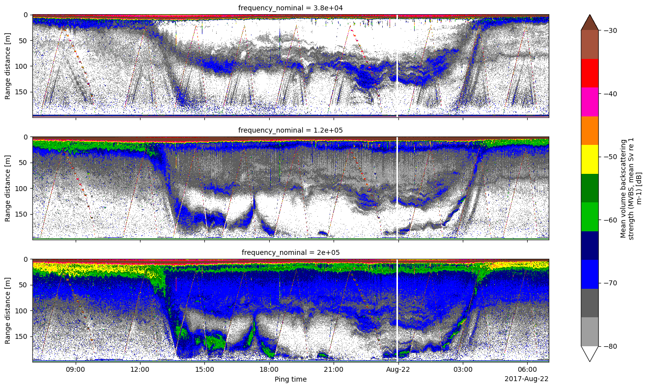
Next we want to compute mean volume backscattering strength (MVBS), which are binned averages of Sv (in the linear domain) across ping time and depth. This gets the echo data onto a common grid that is convenient for visualization and various computation.
Since the binning process can be computationally expensive due to the underlying group_by operation that requires checking the ping_time and depth coordinate values, let’s save and lazy-load the Sv dataset back to make the computation more manageable even on a machine with smaller resources.
for var in ds_Sv.data_vars:
    if "chunks" in ds_Sv[var].encoding:
        ds_Sv[var].encoding.pop("chunks")
    if "preferred_chunks" in ds_Sv[var].encoding:
        ds_Sv[var].encoding.pop("preferred_chunks")
%%time

# Save to Zarr and offload computation to disk
ds_Sv.chunk({"channel": 1, "ping_time": 1000, "range_sample": -1}).to_zarr(
    combined_zarr_path / "ds_Sv.zarr",
    mode="w",
    compute=True,
)

# Lazy-load the Zarr store
ds_Sv = xr.open_dataset(
    combined_zarr_path / "ds_Sv.zarr",
    engine="zarr",
    chunks={},
)
CPU times: total: 13.4 s
Wall time: 22.7 s
Regrid calibrated Sv data to MVBS#
Now we can compute MVBS by leveraging Dask’s distributed computing capability, by specifying the computation on the lazy-loaded Sv dataset first, and save the MVBS output to disk, which forces the computation to happen in a distributed manner.
%%time

# Compute MVBS
ds_MVBS = ep.commongrid.compute_MVBS(
    ds_Sv,
    range_var="depth",
    range_bin="0.5m",
    ping_time_bin="10s",
    reindex=False,
    fill_value=np.nan,
)

# Save to Zarr and offload computation to disk
ds_MVBS.to_zarr(
    combined_zarr_path / "ds_MVBS.zarr",
    mode="w",
    compute=True,
)

# Lazy-load the Zarr store
ds_MVBS = xr.open_dataset(
    combined_zarr_path / "ds_MVBS.zarr",
    engine="zarr",
    chunks={},
)
CPU times: total: 14 s
Wall time: 1min
The resulting MVBS Dataset has a coherent depth coordinate across all frequencies.
ds_MVBS
<xarray.Dataset> Size: 106MB
Dimensions:            (channel: 3, ping_time: 11017, depth: 400)
Coordinates:
  * channel            (channel) object 24B 'GPT  38 kHz 00907208dd13 5-1 OOI...
  * ping_time          (ping_time) datetime64[ns] 88kB 2017-08-21T04:57:10 .....
  * depth              (depth) float64 3kB 0.0 0.5 1.0 1.5 ... 198.5 199.0 199.5
Data variables:
    frequency_nominal  (channel) float64 24B dask.array<chunksize=(1,), meta=np.ndarray>
    Sv                 (channel, ping_time, depth) float64 106MB dask.array<chunksize=(3, 11017, 400), meta=np.ndarray>
Attributes:
    processing_software_name:     echopype
    processing_software_version:  0.11.2.dev12+ge13b48180
    processing_time:              2026-05-11T14:28:55+00:00
processing_function: commongrid.compute_MVBSReplace the channel dimension and coordinate with the frequency_nominal variable containing actual frequency values. Note that this step is possible only when there are no duplicated frequencies present.
ds_MVBS = ep.consolidate.swap_dims_channel_frequency(ds_MVBS)
We can plot it!
import matplotlib as mpl
import echopype.colormap

ds_MVBS["Sv"].sel(
    ping_time=slice(start_datetime, end_datetime)
).plot(
    x="ping_time",
    y="depth",
    col="frequency_nominal",
    col_wrap=1,
    vmin=-80,
    vmax=-30,
    cmap=mpl.colormaps["ep.ek500"],
    yincrease=False,
    figsize=(14, 8),
)
<xarray.plot.facetgrid.FacetGrid at 0x2a6b008a3f0>
Visualize MVBS interactively using hvPlot#
Below you can see that hvPlot gives us a slider for the frequencies for free!
Note: interactive hvplot outputs may not render in the static version of the echopype-examples notebook, but will display correctly when the notebook is run locally.
ds_MVBS["Sv"].hvplot.image(
    x="ping_time", y="depth",
    color="Sv", rasterize=True,
    cmap="jet", clim=(-80, -30),
    xlabel="Time (UTC)",
    ylabel="Depth (m)",
).options(width=800, invert_yaxis=True)
Note that the reflection from the sea surface shows up at a location below the depth of 0 m. This is because we have not corrected for the actual depth of the platform on which the echosounder is mounted, and the actual sound speed at the time of data collection (which is related to the calculated range) could also be different from the user-defined sound speed stored in the data file. More accurate platform depth information can be obtained using data from the CTD collocated on the moored platform.
Obtain solar radiation data from an OOI THREDDS server#
Now we have the sonar data ready, the next step is to pull solar radiation data collected by a nearby surface mooring.
metbk_url = (
    "http://thredds.dataexplorer.oceanobservatories.org/thredds/dodsC/ooigoldcopy/public/"
    "CE04OSSM-SBD11-06-METBKA000-recovered_host-metbk_a_dcl_instrument_recovered/"
    "deployment0004_CE04OSSM-SBD11-06-METBKA000-recovered_host-metbk_a_dcl_instrument_recovered_20170421T022518.003000-20171013T154805.602000.nc#fillmismatch"
)
Let’s quickly take a look at this dataset and decide how to slice it:
xr.open_dataset(metbk_url)
<xarray.Dataset> Size: 280MB
Dimensions:                                   (obs: 252807)
Coordinates:
  * obs                                       (obs) int32 1MB 0 1 ... 252806
    time                                      (obs) datetime64[ns] 2MB ...
Data variables: (12/94)
    northward_wind_velocity_qc_executed       (obs) uint8 253kB ...
    air_temperature_qc_results                (obs) uint8 253kB ...
    northward_wind_velocity                   (obs) float32 1MB ...
    precipitation                             (obs) float32 1MB ...
    sea_surface_conductivity_qc_executed      (obs) uint8 253kB ...
    sea_surface_temperature_qartod_executed   (obs) |S64 16MB ...
    ...                                        ...
    sea_surface_temperature_qartod_results    (obs) uint8 253kB ...
    precipitation_qc_executed                 (obs) uint8 253kB ...
    northward_wind_velocity_qc_results        (obs) uint8 253kB ...
    met_relwind_speed                         (obs) float64 2MB ...
    met_netsirr_qc_results                    (obs) uint8 253kB ...
    relative_humidity_qartod_executed         (obs) |S64 16MB ...
Attributes: (12/73)
    node:                               SBD11
    comment:
    publisher_email:
    sourceUrl:                          http://oceanobservatories.org/
    collection_method:                  recovered_host
    stream:                             metbk_a_dcl_instrument_recovered
    ...                                 ...
    geospatial_vertical_positive:       down
    lat:                                44.36555
    lon:                                -124.9407
    DODS.strlen:                        36
    DODS.dimName:                       string36
DODS_EXTRA.Unlimited_Dimension: obsmetbk_ds = (
xr.open_dataset(metbk_url)
.swap_dims({"obs": "time"})
.drop_vars("obs")
.sel(time=slice(start_datetime, end_datetime))[["shortwave_irradiance"]]
)
metbk_ds["time"].attrs.update({"long_name": "Time", "units": "UTC"})
metbk_ds
<xarray.Dataset> Size: 17kB
Dimensions:               (time: 1441)
Coordinates:
  * time                  (time) datetime64[ns] 12kB 2017-08-21T07:00:08.2329...
Data variables:
    shortwave_irradiance  (time) float32 6kB ...
Attributes: (12/73)
    node:                               SBD11
    comment:
    publisher_email:
    sourceUrl:                          http://oceanobservatories.org/
    collection_method:                  recovered_host
    stream:                             metbk_a_dcl_instrument_recovered
    ...                                 ...
    geospatial_vertical_positive:       down
    lat:                                44.36555
    lon:                                -124.9407
    DODS.strlen:                        36
    DODS.dimName:                       string36
DODS_EXTRA.Unlimited_Dimension: obsPlot the echosounder and solar radiation data together to visualize zooplankton response to a solar eclipse#
We can finally put everything together and figure out the impact of the eclipse-driven reduction in sunlight on marine zooplankton!
import matplotlib.pyplot as plt

fig = plt.figure(figsize=(14, 7))

gs = fig.add_gridspec(
    2, 2,
    width_ratios=[30, 1],
    height_ratios=[1, 3],
    hspace=0.05,
    wspace=0.08,
)

ax_top = fig.add_subplot(gs[0, 0])
ax_bottom = fig.add_subplot(gs[1, 0], sharex=ax_top)
cax = fig.add_subplot(gs[1, 1])

# Top plot
metbk_ds["shortwave_irradiance"].plot(
    ax=ax_top,
    x="time",
)
ax_top.set_yscale("log")
ax_top.set_xlim(start_datetime, end_datetime)
ax_top.set_ylabel("Downwelling\nshortwave irradiance")
ax_top.set_xlabel("")
ax_top.set_title("")
ax_top.tick_params(labelbottom=False)

# Bottom echogram
ds_MVBS["Sv"].sel(
    frequency_nominal=200000,
    ping_time=slice(start_datetime, end_datetime),
).plot(
    ax=ax_bottom,
    x="ping_time",
    y="depth",
    cmap=mpl.colormaps["ep.ek500"],
    vmin=-80,
    vmax=-30,
    yincrease=False,
    cbar_ax=cax,
)

ax_bottom.set_title("")
ax_bottom.set_xlabel("Time (UTC)")
ax_bottom.set_ylabel("Depth (m)")

plt.show()
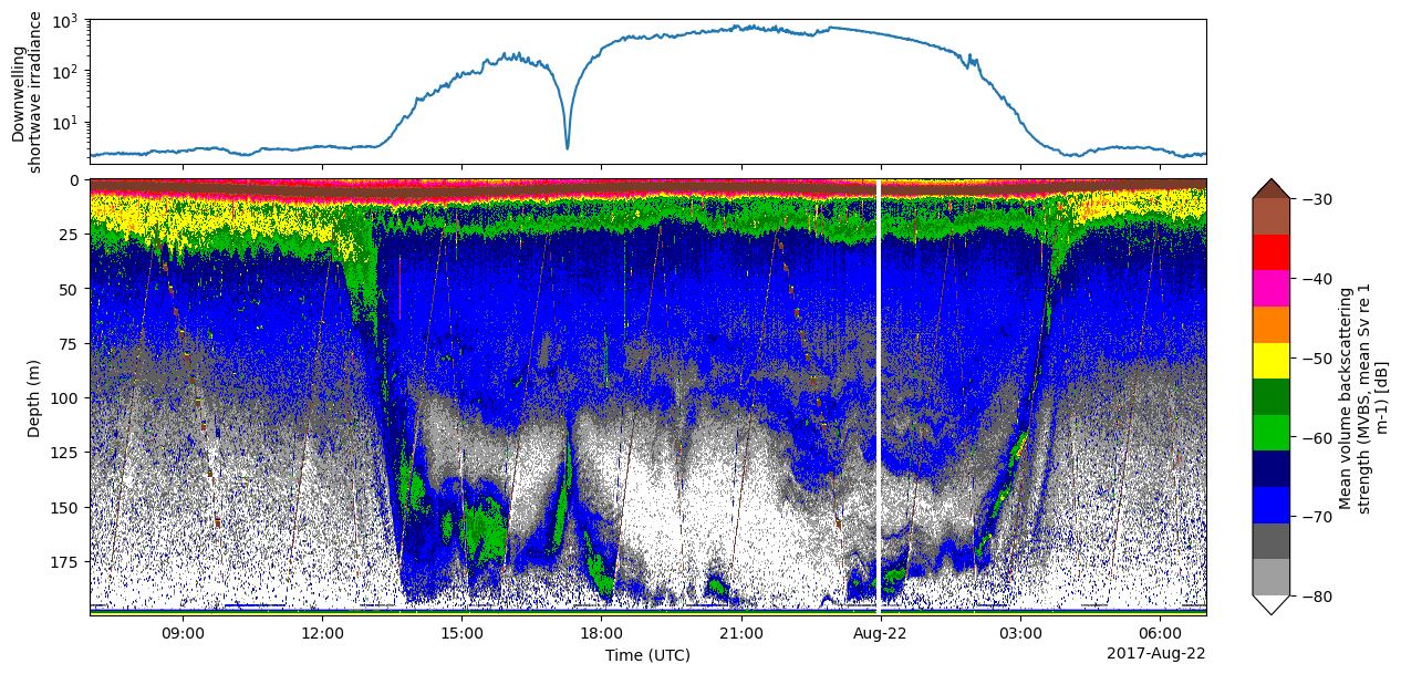
Look how the dip at solar radiation reading matches exactly with the upwarding moving “blip” at UTC 17:21, August 22, 2017 (local time 10:22 AM). During the solar eclipse, the animals were fooled by the temporary mask of the sun and thought it’s getting dark as at dusk!
As previously, we can also explore this relationship interactively using hvplot.
Note: as mentioned above, interactive hvplot outputs may not render in the static notebook preview.
metbk_plot = metbk_ds.hvplot.line(
    x="time", y="shortwave_irradiance",
).options(width=800, height=200, logy=True, xlim=(start_datetime, end_datetime))

mvbs_plot = ds_MVBS["Sv"].sel(frequency_nominal=200000, ping_time=slice(start_datetime, end_datetime)).hvplot.image(
    x="ping_time", y="depth",
    color="Sv", rasterize=True,
    cmap="jet", clim=(-80, -30),
    xlabel="Time (UTC)",
    ylabel="Depth (m)"
).options(width=800, invert_yaxis=True).redim(x="ping_time")
(metbk_plot + mvbs_plot).cols(1)
Package versions#
import datetime
print(f"echopype: {ep.__version__}, xarray: {xr.__version__}, fsspec: {fsspec.__version__}, "
      f"hvplot: {hvplot.__version__}")

print(f"\n{datetime.datetime.now(datetime.timezone.utc).isoformat()}")
echopype: 0.11.2.dev12+ge13b48180, xarray: 2026.4.0, fsspec: 2026.4.0, hvplot: 0.12.2

2026-05-11T14:34:02.847252+00:00